T Coronae Borealis (T CrB for short) is a variable star in the constellation Corona Borealis (the northern crown). Historically, it has undergone nova outbursts and is expected to undergo another one soon.
In[]:=
Withstar=,AstroGraphics[{Red,Point[star],White,Text["T CrB",star,{0,1.5}]},AstroReferenceFrame->"Equatorial",AstroBackground->AstroStyling[{"BlackSky","ShowConstellationIllustrations"->True,"ConstellationIllustrationStyle"->Directive[Opacity[.03],White,EdgeForm[Directive[Opacity[.15],Darker[Gray,.1]]]]}]]
Out[]=
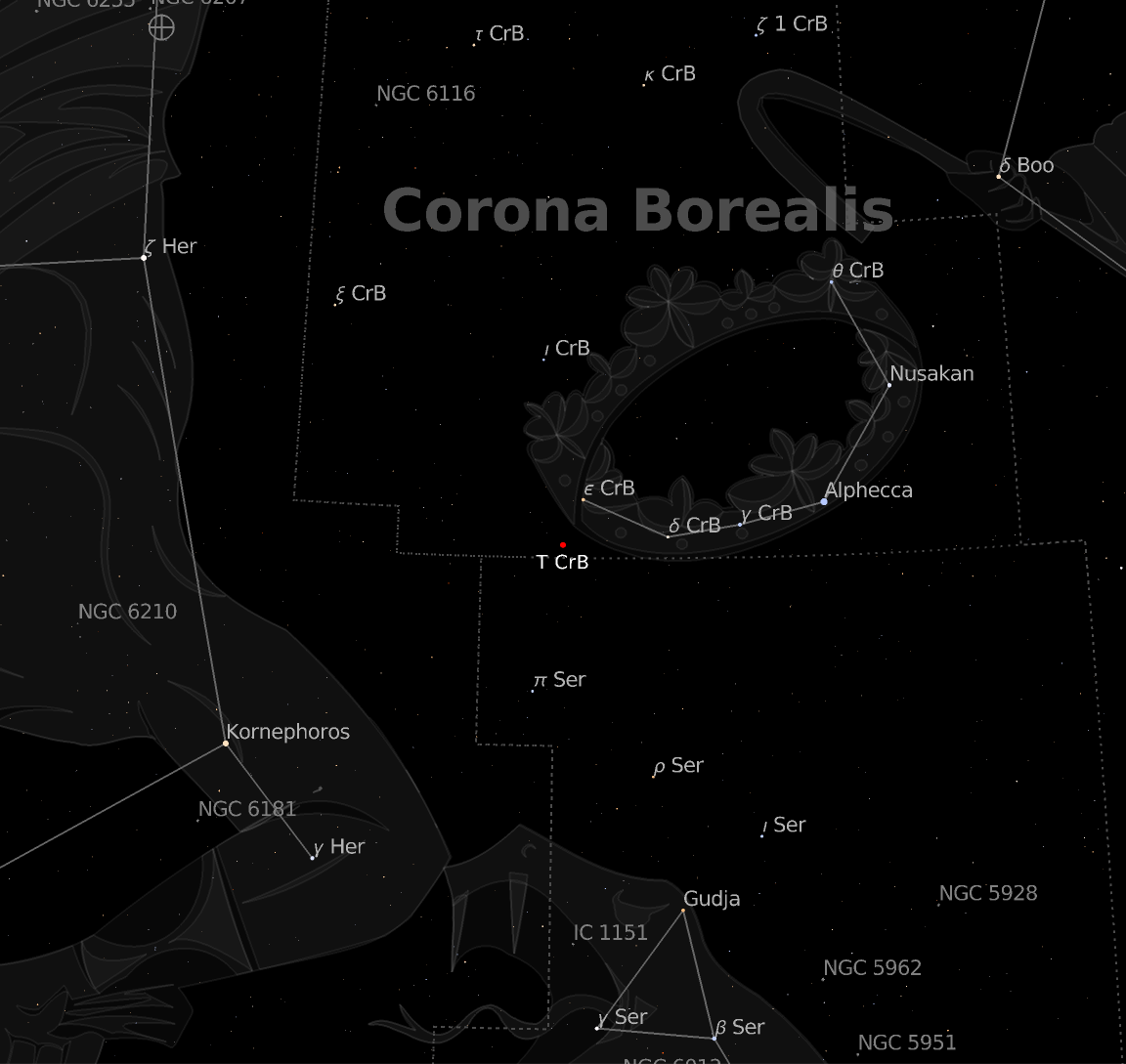
Typically this star system is relatively obscure with an apparent magnitude hovering around 10.8, but as with all variable stars, things can change. T CrB is known to be a recurrent nova, a specific type of cataclysmic variable star that undergoes nova outbursts periodically. When in outburst, the star system brightens from magnitude 10.8 all the way up to magnitude 2, nearly 9 orders of magnitude brighter! Though even between outbursts, the brightness of the system oscillates on smaller scales due to short term orbital effects such as the face of the secondary star being heated by the primary star and an accretion disk.
In[]:=
EntityValue,,,,,,,"Dataset"
Out[]=
The period between these outbursts is about 79 years.
In[]:=
UnitConvert["VariablePeriod"],"Years"
Out[]=
The reason for the recent media coverage of T CrB in March 2023 is that the system seems to be dimming systematically, an event that was a precursor to the last outburst in 1946 (about 77 years ago). T Coronae Borealis may be preparing to undergo another nova outburst and could become as bright as Polaris, the north star. Polaris is the brightest star in the constellation Ursa Minor (the little dipper), but it’s nowhere near the brightest star in the sky. Polaris ranks about 49th in the list of brightest stars in the night sky, so it’s far from being the brightest star in the sky, but still easily visible in all but the most light polluted skies.
We can plot the recent brightness variations of T CrB by analyzing AAVSO light curve data.
In[]:=
tdb=ResourceFunction["AAVSOLightCurveData"],<|"Filters"->"B","DateRange"->{DateObject[{2022,1,1}],DateObject[{2024,3,23}]}|>,"TemporalData"
Out[]=
TemporalData


Plot the B (blue) filter brightness measurements with a 7 day median filtered form on top to clean things up a bit.
In[]:=
DateListPlot[{tdb,MovingMap[Median,tdb,Quantity[7,"Days"]]},ScalingFunctions->{None,"Reverse"},PlotRange->{10,12.5},PlotStyle->{SetAlphaChannel[ColorData[97][1],.2],ColorData[97][2]}]
Out[]=
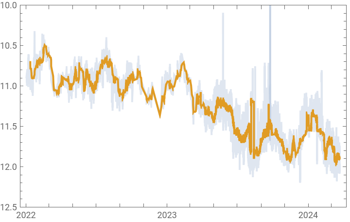
Starting in early 2023, the overall trend of the normal variations was downwards, dropping from about magnitude 10.8 and approaching magnitude 12. This could indicate a precursor to a nova outburst based on similar behavior observed in 1946 during the last outburst.
Computation and Visualization
Computation and Visualization
The shape of the secondary star is determined by the shape of one Roche lobe of the gravitational potential which, in turn, is determined by parameters such as the mass ratio of the stars and the orbital period . The potential function can be defined as follows.
()
P
orb
-+x-μ+-++-++
1
2
2
aq
q+1
2
y
2
Ω
orb
Gq
M
1
2
-a+x+
q
q+1
2
y
2
z
G
M
1
2
+x
q
q+1
2
y
2
z
where a is the distance separating the stars, q is the mass ratio, is the mass of the primary star, is 2 , G is the universal gravitational constant.
M
1
Ω
orb
π/
P
orb
Because the secondary star overflows its Roche lobe, matter is lost to the star and it is transferred to the primary star. The path of a gas particle ejected from the secondary star through the first Lagrange point follows the equations of motion of the restricted three body problem. The location of three Lagrange points can be found by solving for the roots of the potential function along the x-axis. By solving for the first Lagrange point, we locate the initial starting point of the particle stream.
The equations of motion for the restricted three-body problem can be described as follows. These describe the motion of a gas particle affected only by gravitational and rotational effects, magnetic fields and friction are ignored. We will use NDSolve to solve the equations up to the point that the mass transfer stream impacts the edge of the accretion disk.
′′
x
μ(μ+x(t)-1)
3/2
+
2
(μ+x(t)-1)
2
y(t)
′
y
(1-μ)(μ+x(t))
3/2
+
2
(μ+x(t))
2
y(t)
′′
y
μy(t)
3/2
+
2
(μ+x(t)-1)
2
y(t)
(1-μ)y(t)
3/2
+
2
(μ+x(t))
2
y(t)
′
x
where q = μ/(1-μ)
To simulate the T CrB system, we need to know some physical parameters of the star system. The primary star is a massive white dwarf star of about 1.37 solar masses. This mass is not far from the Chandrasekhar limit (~1.4 solar masses), so given enough time and mass accretion, it’s possible T CrB is a precursor for becoming a Type Ia supernova one day if it ever accretes enough matter from the secondary star to exceed that limit. The secondary star, orbiting about 0.54 AU away with a period of about 227 days, is a red giant star of about 1.12 solar masses that fills its Roche lobe and thus initiates mass transfer to the primary star where an accretion disk forms. When enough hydrogen from the secondary star accumulates on the white dwarf surface, it gets heated to the point that a runaway fusion reaction of this hydrogen begins and a nova is born. In the case of T CrB, these novae outbursts repeat about every 79 years or so.
We set up some initial conditions such as the mass ratio of the system (q), the mass of the primary object/star (M1), the initial velocities of the mass transfer stream, and various other computations. The shape of the red giant star is constrained by the gravitational potential of the system and fills its Roche lobe. The following solves for the various Lagrange points, especially the L1 point, using the L2 and L3 points as plot range constraints.
In[]:=
q=1.37/1.12;M1=1.37;M2=q*M1;μpotential=M2/(M1+M2);a=1;G=1;Porb=Sqrt[4*Pi^2*(a^3/(G*(1+q)))];Ωorb=2*(Pi/Porb);
In[]:=
Φ[x_,y_,z_]:=-((G*M1)/Sqrt[(x+q/(1+q))^2+y^2+z^2])-(G*M2)/Sqrt[(x-a+q/(1+q))^2+y^2+z^2]-(1/2)*Ωorb^2*((x-μpotential+(q/(1+q))*a)^2+y^2);
In[]:=
deriv=D[Φ[x,0,0],x];posAtL1=FindRoot[deriv==0,{x,.3}];ΦAtL1=Φ[x/.posAtL1,0,0];posAtL2=FindRoot[deriv==0,{x,1.5}];ΦAtL2=Φ[x/.posAtL2,0,0];posAtL3=FindRoot[deriv==0,{x,-1}];ΦAtL3=Φ[x/.posAtL3,0,0];
The position of the white dwarf is found at {-μ,0,0}.
In[]:=
μ=mu/.Quiet[Solve[q==mu/(1-mu),mu],Solve::ratnz][[1]];
The surface of the red giant is generated using the following.
In[]:=
grL1=ContourPlot3D[Φ[x,y,z],{x,x/.posAtL1,x/.posAtL2},{y,-0.7,0.7},{z,-0.6,0.6},Contours->{ΦAtL1},ContourStyle->{RGBColor[1,.3,0]},Mesh->None,Lighting->{AmbientLight[GrayLevel[.7]],PointLight[White,{-μ,0,0}]}];
In[]:=
mypr={{(x/.posAtL3),x/.posAtL2},{-.5,.5},{-0.6,0.6}};
The accretion disk is represented using a textured 3D disk centered on the white dwarf at {-μ,0,0}.
In[]:=
texture=ColorReplace
,Black->RGBColor[0,0,0,0];

In[]:=
pdisk[mu_,rad_]:=ParametricPlot3D[{rCos[t]-mu,rSin[t],0},{r,.02,rad},{t,0,2π},PlotPoints75,PlotRange{Automatic,Automatic,{-.1,.1}},ImageSize600,PlotStyle->Texture[texture],TextureCoordinateFunction->({#1,#2}&),Mesh->None,Lighting->{DirectionalLight[GrayLevel[.35],{0,0,1}],DirectionalLight[GrayLevel[.35],{0,0,-1}]}]
The radius of the accretion disk in quiescence is relatively small, estimated to be about 6 solar radii, set here to .05 times the semimajor axis. In scaled units of the semimajor axis, we have:
In[]:=
diskrad=Quantity[6,"SolarRadius"]/Quantity[.54,"AstronomicalUnit"]
Out[]=
0.0516719
The inclination of the system was estimated to be about 67° according to V. Stanishev et al (2003). This estimate is bounded by the fact that the system isn’t eclipsing so can’t be higher than about 70° and if it’s less than about 65° the derived mass of the white dwarf would exceed the Chandrasekhar limit.
In[]:=
inclination=67;
We can solve for the trajectory of the mass transfer stream leaving the first Lagrange point of the system and falling towards the white dwarf. The stream should impact the accretion disk at a point that can be determined via event detection.
In[]:=
Vx0=-0.01;Vy0=0.00333300000000002;
In[]:=
event[x_,y_,t_,drad_]:=WhenEvent[N[Norm[{x[t]+μ,y[t],0}]]drad,Sow[t];"StopIntegration"]
In[]:=
eqs[x_,y_,t_,drad_]:=[t]2[t]+x[t]--,[t]-2[t]+y[t]--,y[0]0,x[0]Evaluate[x/.posAtL1],[0]Vy0,[0]Vx0,event[x,y,t,drad];
′′
x
′
y
(1-μ)(x[t]+μ)
3/2
(+)
2
(x[t]+μ)
2
y[t]
μ(x[t]-1+μ)
3/2
(+)
2
(x[t]-1+μ)
2
y[t]
′′
y
′
x
(1-μ)y[t]
3/2
(+)
2
(x[t]+μ)
2
y[t]
μy[t]
3/2
(+)
2
(x[t]-1+μ)
2
y[t]
′
y
′
x
So that the impact point can be easily extracted from the InterpolatingFunction returned by NDSolve, we load an additional package that makes this possible.
The point where the mass transfer stream impacts the accretion disk is the location of a bright spot as the infalling gas changes velocity and is shocked.
Here is a graphics representation of the mass transfer stream.
We can visualize the system by specifying the orbital phase. The white dwarf is tiny, on the order of .01 solar radii, so would be difficult to see if rendered to scale, so its size is magnified here.
References
References
V. Stanishev et. al., Hα variability of the recurrent nova T Coronae Borealis, A&A 415, 609-616 (2004)
Warner,B. Cataclysmic Variable Stars. Cambridge,England:Cambridge University Press,1995.
CITE THIS NOTEBOOK
CITE THIS NOTEBOOK
T Coronae Borealis - about to go nova....again
by Jeffrey Bryant
Wolfram Community, STAFF PICKS, March 24, 2024
https://community.wolfram.com/groups/-/m/t/3146524
by Jeffrey Bryant
Wolfram Community, STAFF PICKS, March 24, 2024
https://community.wolfram.com/groups/-/m/t/3146524