Basically every day there are NASA Perseverance Mars Rover new images from Mars, kindly shared and published.
And of course we can compute it and do some data science on it.
I am wondering where are those places on Earth that seams to be like Mars landscape?
We can get a NASA published Mars rover image and use against geo location neural network and figure it out!
And of course we can compute it and do some data science on it.
I am wondering where are those places on Earth that seams to be like Mars landscape?
We can get a NASA published Mars rover image and use against geo location neural network and figure it out!
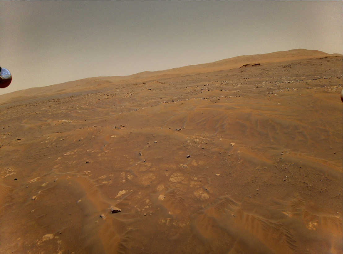
First, get one Mars image from NASA website, I just did a copy, past to my notebook:
In[]:=
marsImg=
;
In[]:=
Information[marsImg]
Out[]=
In[]:=
ImageDimensions[marsImg]
Out[]=
{1600,1186}
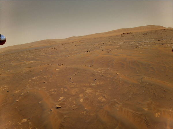
Reduce image size for this example. But in research it is good to work with the full image resolution...
In[]:=
marsImg=ImageResize[marsImg,600]
Out[]=
In[]:=
ImageDimensions[marsImg]
Out[]=
{600,445}
Now import a ready to use neural network from Wolfram Neural Network Repository that can give as a geo location based in a photo:
In[]:=
locationNn=NetModel["ResNet-101 Trained on YFCC100m Geotagged Data"]
Out[]=
NetChain


Use Mars image as input and check the geo location on Earth
In[]:=
position=locationnn[marsImg]
Out[]=
GeoPosition[{31.1058,8.48245}]
Visualize the area with this geo location (latitude, longitude):
In[]:=
GeoGraphics[position]
Out[]=
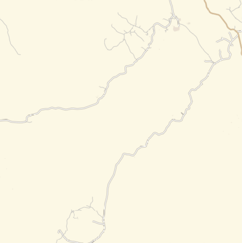
Well it is in a desert, distant from urban areas...
Lets take a closer look...
Lets take a closer look...
GeoGraphicsGeoDiskposition,
Out[]=

Well it does not tell much where it is...
Lets zoom out...
Lets zoom out...
In[]:=
GeoGraphicsGeoDiskposition,,GeoRangeQuantity[10,"Kilometers"]
Out[]=
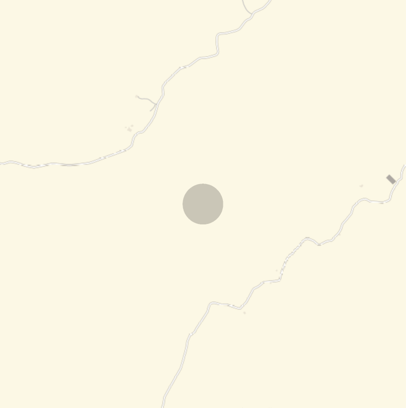
Zoom out more, geo disk about 100km and geo range of 1000km:
OK, lest zoom out more...
Now we can check more probable landscapes on Earth that is similar to Mars according the image given...
For another test, we can view the Mars image as black and white.
And we can try to colorize it artificially with a neural network too trained with Earth images.
And we can try to colorize it artificially with a neural network too trained with Earth images.
This function convert the neural network output data back in a image, this source code is available at the repository too:
Now lest see side by side the original Mars image, the grey scale and the artificially colored image:
Of course a dessert landscape on Earth probably would have a beautiful clean blue sky, the ground is really close from the original Mars image.
Lest see where this artificial colored Mars image can be seen on Earth:
We can check some info about this neural network we are using to get geo location from an given image:
Another visualization, with colored dots at each geo location, hue color adjusted as the probabilities: