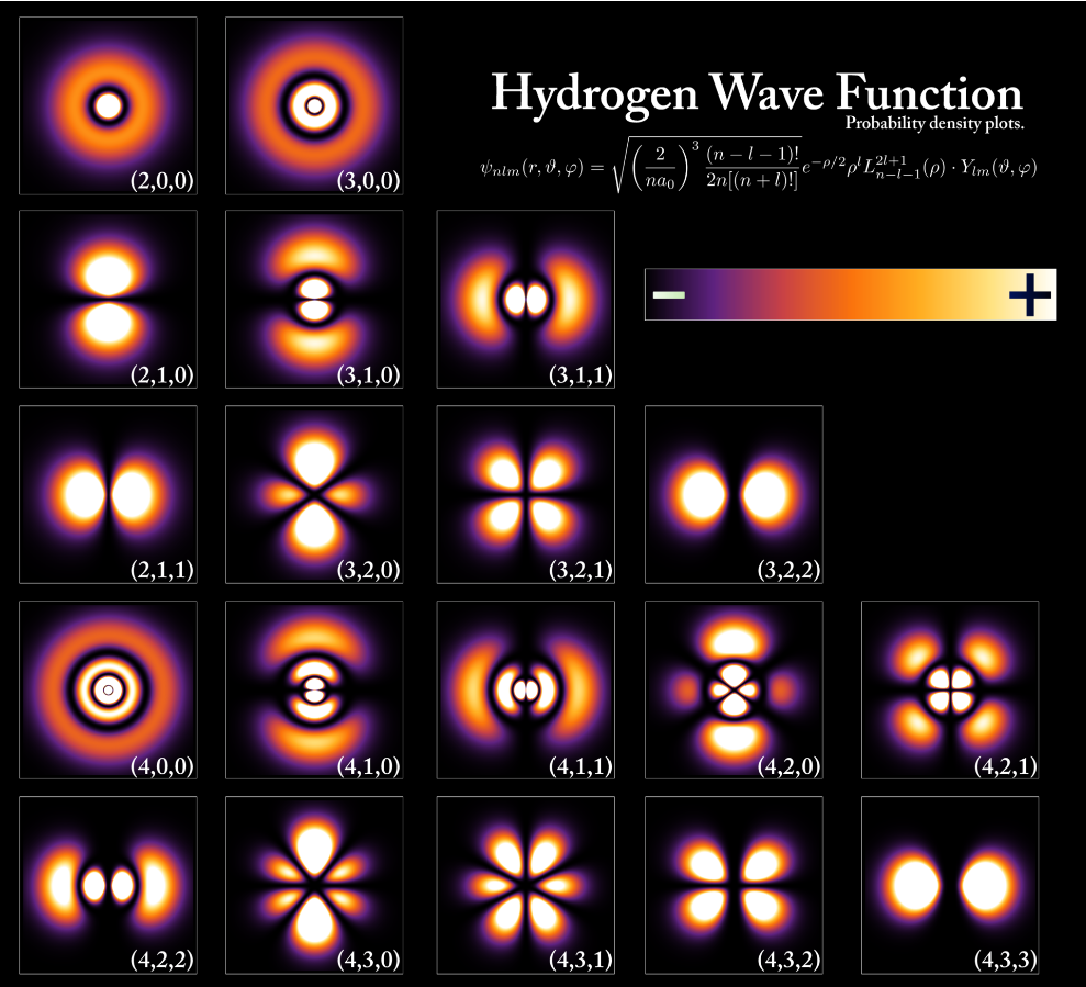
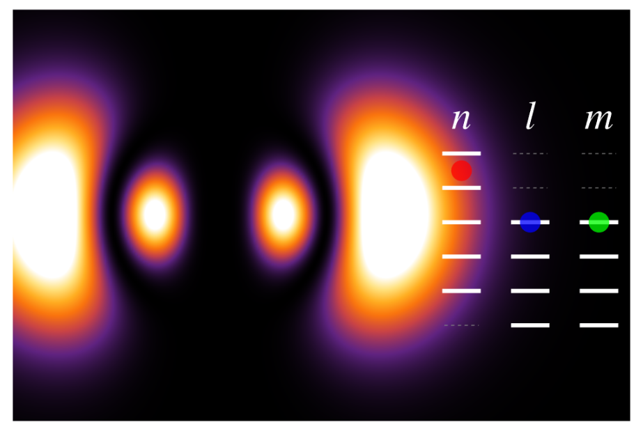
This animation shows the spatial probability density of finding an electron in a hydrogen atom. The Hydrogen wavefunctions transitioning between states with different quantum numbers 𝒏,𝒍,𝒎. The quantum numbers 𝒏,𝒍,𝒎 are the parameters which specify the state of the hydrogen atom:
• 𝒏: total energy
• 𝒍: total angular momentum
• 𝒎: z-component of angular momentum
Each transition shows a state α|𝒏𝒍𝒎⟩ + β|𝒏’𝒍’𝒎’⟩, where α decreases and β increases. Dots represent the values of 𝒏𝒍𝒎, and the solid lines show possible allowed values.
• 𝒏: total energy
• 𝒍: total angular momentum
• 𝒎: z-component of angular momentum
Each transition shows a state α|𝒏𝒍𝒎⟩ + β|𝒏’𝒍’𝒎’⟩, where α decreases and β increases. Dots represent the values of 𝒏𝒍𝒎, and the solid lines show possible allowed values.
Full code
Full code
In[]:=
<<MaTeX`SetOptions[MaTeX,"Preamble"{"\\usepackage{color,txfonts}"}];SetDirectory[NotebookDirectory[]];
In[]:=
Clear[drawLadder];drawLadder[n_,l_,m_,imsize_:500]:=Module[{maxrungs=5,mag=4},Graphics[{White,Opacity[1],Thickness[.02],Dashing[None],Table[Line[{{0,k},{1,k}}],{k,maxrungs}],(*drawnlines*)Gray,Dashed,Thickness[.005],Line[{{0,0},{1,0}}],Red,Opacity[.75],Disk[{0.5,n},.3],White,Opacity[1],Thickness[.02],Dashing[None],Table[Line[{{2,k},{3,k}}],{k,0,Floor[n+0.01]-1}],(*drawllines*)Gray,Dashed,Thickness[.005],Table[Line[{{2,k},{3,k}}],{k,Floor[n+0.01],maxrungs}],Blue,Opacity[.75],Disk[{2.5,l},.3],White,Opacity[1],Thickness[.02],Dashing[None],Table[Line[{{4,k},{5,k}}],{k,0,Ceiling[l-0.01]}],(*drawmlines*)Gray,Dashed,Thickness[.005],Table[Line[{{4,k},{5,k}}],{k,Ceiling[l-0.01]+1,maxrungs}],Green,Opacity[.75],Disk[{4.5,m},.3],White,Opacity[1],Thick,Dashing[None],Text[MaTeX["\\color{white} n",Magnificationmag],{.5,maxrungs+1}],Text[MaTeX["\\color{white} l",Magnificationmag],{2.5,maxrungs+1}],Text[MaTeX["\\color{white} m",Magnificationmag],{4.5,maxrungs+1}],Table[Text[MaTeX["\\color{white} "<>ToString[k],Magnification.5*mag],{5.8,k}],{k,0,maxrungs}]},(*BackgroundBlack,*)BackgroundTransparent,ImageSizeimsize]];(*drawLadder[3,2,0]*)
Clear[drawFrame];drawFrame[{n1_,l1_,m1_},{n2_,l2_,m2_},c1_,c2_]:=Module{c1norm,c2norm},c1norm=c1+;c2norm=c2+;ListDensityPlotTableModule{r=Norm[{x,0,z}],eq1,eq2},eq1=LaguerreLn1-1-l1,2l1+1,SphericalHarmonicYl1,m1,ArcCos,ArcTan[x,0];eq2=LaguerreLn2-1-l2,2l2+1,SphericalHarmonicYl2,m2,ArcCos,ArcTan[x,0];,{z,-40.1,40,.5},{x,-40.1,80,.5},DataRange{{-40,40},{-40,80}},AspectRatio.81.2,ImageSize1000*{1.2,.8},MeshFalse,FrameFalse,ColorFunctionScalingTrue,ColorFunction"SunsetColors",EpilogInset[drawLadder[n1*c1norm^2+n2*c2norm^2,l1*c1norm^2+l2*c2norm^2,m1*c1norm^2+m2*c2norm^2,250],{29,20}](*drawFrame[{4,3,3},{5,3,3},.5,.5]*)
2
Abs[c1]
2
Abs[c2]
2
Abs[c1]
2
Abs[c2]
4π
rExp-r
n1
l1
r
2r
n1
z
r
4π
rExp-r
n2
l2
r
2r
n2
z
r
2
Abs[c1norm*eq1+c2norm*eq2]
Out[]=
Clear[renderFrame];renderFrame[t_]:=Module[{tt=t-Floor[t],c1,c2,ttt},ttt=Piecewise[{{0,tt<.1},{(tt-.1)/(1-.1-.1),.1≤tt<.9},{1,tt≥.9}}];c1=Cos[π/2*ttt];c2=Sin[π/2*ttt];Switch[Floor[t],0,drawFrame[{5,0,0},{4,0,0},c1,c2],1,drawFrame[{4,0,0},{3,0,0},c1,c2],2,drawFrame[{3,0,0},{3,1,0},c1,c2],3,drawFrame[{3,1,0},{3,1,1},c1,c2],4,drawFrame[{3,1,1},{4,0,0},c1,c2],5,drawFrame[{4,0,0},{4,1,1},c1,c2],6,drawFrame[{4,1,1},{4,2,1},c1,c2],7,drawFrame[{4,2,1},{4,3,1},c1,c2],8,drawFrame[{4,3,1},{5,0,0},c1,c2],9,drawFrame[{5,0,0},{5,1,1},c1,c2],10,drawFrame[{5,1,1},{5,2,1},c1,c2],11,drawFrame[{5,2,1},{5,3,1},c1,c2],12,drawFrame[{5,3,1},{5,4,1},c1,c2],13,drawFrame[{5,4,1},{5,3,1},c1,c2],14,drawFrame[{5,3,1},{5,2,1},c1,c2],15,drawFrame[{5,2,1},{5,1,1},c1,c2],16,drawFrame[{5,1,1},{4,1,1},c1,c2],17,drawFrame[{4,1,1},{3,1,1},c1,c2],18,drawFrame[{3,1,1},{2,1,1},c1,c2],19,drawFrame[{2,1,1},{1,0,0},c1,c2],_,drawFrame[{2,1,0},{1,0,0},0,1]]];(*renderFrame[0.9]*)
In 3D
In 3D
CITE THIS NOTEBOOK
CITE THIS NOTEBOOK
Hydrogen wavefunctions transitioning between different states
by Ben Bartlett
Wolfram Community, STAFF PICKS, March 2, 2022
https://community.wolfram.com/groups/-/m/t/2483815
by Ben Bartlett
Wolfram Community, STAFF PICKS, March 2, 2022
https://community.wolfram.com/groups/-/m/t/2483815