I recently needed to investigate graph products. Mathematica has had the GraphProduct function built-in since version 13.1, but I have found it to be a bit slow in my applications. Thus, I looked into how to efficiently implement a graph product, and was sucked into the correspondences between graph products and matrix products, which dovetailed into looking up some of the more exotic ways to combine two matrices.
Let’s start with the usual Cartesian product (sometimes called the “box product”). Consider these two graphs:
In[]:=
g1=
;g2=

;
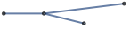
This is the result of combining them with GraphProduct:
In[]:=
gp1=GraphProduct[g1,g2]
Out[]=
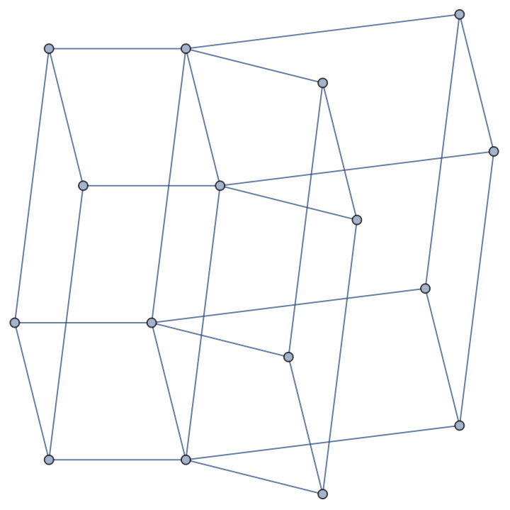
This is equivalent to explicitly specifying the third argument of GraphProduct as “Cartesian”. We can use IsomorphicGraphQ to verify the equivalence:
In[]:=
IsomorphicGraphQ[GraphProduct[g1,g2,"Cartesian"],gp1]
Out[]=
True
In fact, this operation is equivalent to taking an appropriate matrix product of their adjacency matrices. Let’s compute those, using the AdjacencyMatrix function:
In[]:=
a1=AdjacencyMatrix[g1];a2=AdjacencyMatrix[g2];
This visualizes their structure:
In[]:=
MatrixPlot/@{a1,a2}
Out[]=
,
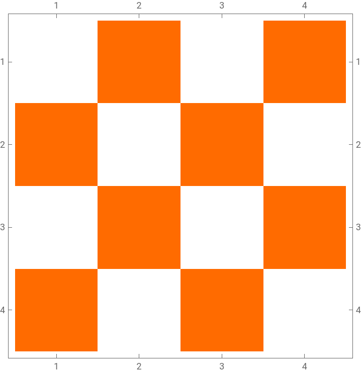
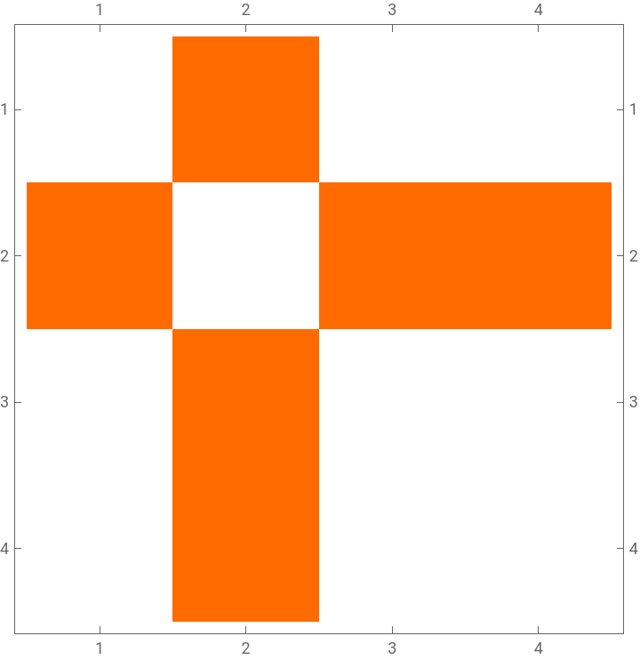
The equivalence needed here is that the Cartesian product of graphs is equivalent to taking the Kronecker sum of their corresponding adjacency matrices. Here is an implementation of the Kronecker sum function:
In[]:=
KroneckerSum[a_?SquareMatrixQ,b_?SquareMatrixQ]:=KroneckerProduct[a,IdentityMatrix[Length[b],SparseArray]]+KroneckerProduct[IdentityMatrix[Length[a],SparseArray],b]
Note that its definition uses the built-in KroneckerProduct function, which is able to cope with the sparse matrices used to represent adjacency matrices of graphs. We can now use the Kronecker sum function, along with the function AdjacencyGraph, to define our own Cartesian product function:
In[]:=
newCartesianProduct[g1_?GraphQ,g2_?GraphQ,opts:OptionsPattern[GraphProduct]]:=With[{m1=AdjacencyMatrix[g1],m2=AdjacencyMatrix[g2]},AdjacencyGraph[KroneckerSum[m1,m2],opts]]
(At this juncture, I should state that these demonstration functions currently do not account for things like annotations or option inheritance; some additional work is necessary if those are important to you.)
Try it out:
In[]:=
gp2=newCartesianProduct[g1,g2]
Out[]=
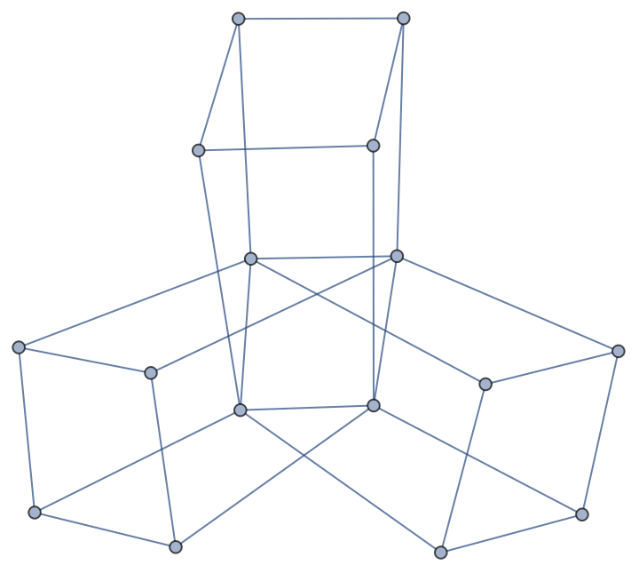
The result of the new function looks a bit different, but we can easily verify the equivalence:
In[]:=
IsomorphicGraphQ[gp1,gp2]
Out[]=
True
As mentioned, the original intent was to come up with a function faster than the built-in GraphProduct. Let’s test that with some medium-sized randomly generated graphs:
In[]:=
gb1=RandomGraph[BarabasiAlbertGraphDistribution[135,2]];gb2=RandomGraph[BarabasiAlbertGraphDistribution[131,2]];
In[]:=
MatrixPlot@*AdjacencyMatrix/@{gb1,gb2}
Out[]=
,
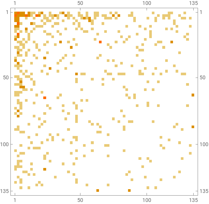
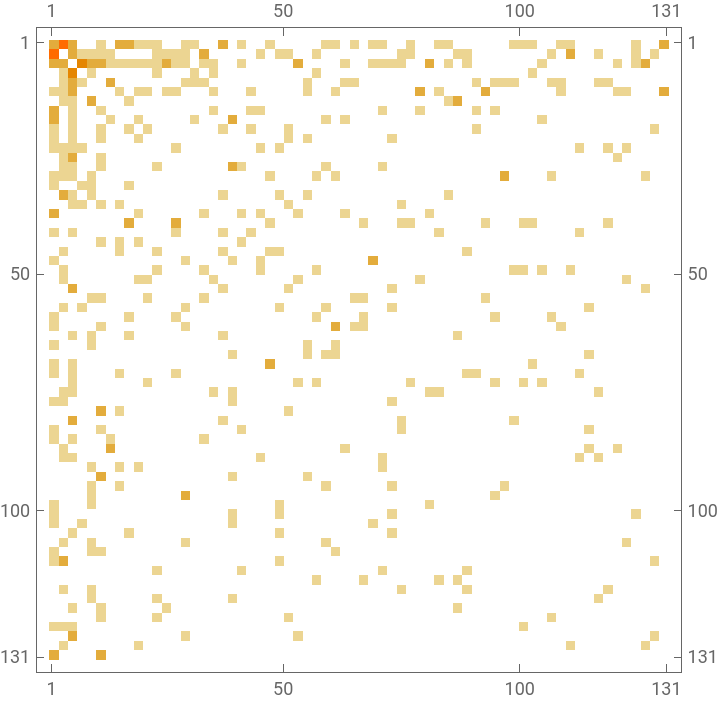
Compare the performance of GraphProduct with the new function:
In[]:=
RepeatedTiming[gpb1=GraphProduct[gb1,gb2,"Cartesian"];]
Out[]=
{11.9377,Null}
In[]:=
RepeatedTiming[gpb2=newCartesianProduct[gb1,gb2];]
Out[]=
{0.845228,Null}
The new function is quite a bit faster, and gives equivalent results:
In[]:=
IsomorphicGraphQ[gpb1,gpb2]
Out[]=
True
In fact, the Kronecker product of two adjacency matrices is itself equivalent to a graph product. This corresponds to the graph tensor product, and can be specified using the string “Tensor” in the third argument of GraphProduct:
In[]:=
gt1=GraphProduct[g1,g2,"Tensor"]
Out[]=
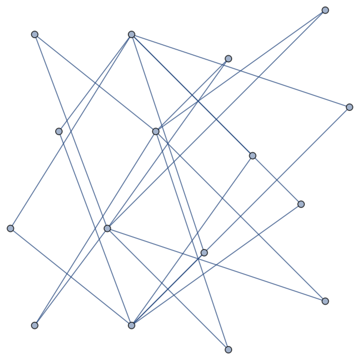
Let’s define our tensor product function:
In[]:=
newTensorProduct[g1_?GraphQ,g2_?GraphQ,opts:OptionsPattern[GraphProduct]]:=With[{m1=AdjacencyMatrix[g1],m2=AdjacencyMatrix[g2]},AdjacencyGraph[KroneckerProduct[m1,m2],opts]]
Again, the result of our new function might look different, but the result is certainly isomorphic to the built-in:
In[]:=
gt2=newTensorProduct[g1,g2]
Out[]=
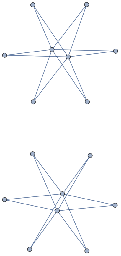
Timing and comparison tests once again favor the new implementation:
Apart from the two graph products already shown, GraphProduct supports four other types of graph product. (In fact, I really only needed the two products above for my purposes, but decided to write something comprehensive for my own and others’ benefit.) It should come as no surprise at this point that these can also be implemented as matrix operations on adjacency matrices. (The observant will notice that all of the efficient definitions rely on KroneckerProduct.) For instance, the lexicographic product (a.k.a. graph composition) can be implemented like so:
We again proceed with a comparison:
Here’s one for the conormal graph product, also known as the “disjunctive product”:
In all cases, the new implementations were much more efficient than the built-in GraphProduct. Hopefully, improvements of this sort can be incorporated in future versions of Mathematica.
CITE THIS NOTEBOOK
CITE THIS NOTEBOOK
On Graph Products and Matrix Products
by J. M.
Wolfram Community, STAFF PICKS, November 22, 2023
https://community.wolfram.com/groups/-/m/t/3069212
by J. M.
Wolfram Community, STAFF PICKS, November 22, 2023
https://community.wolfram.com/groups/-/m/t/3069212