All Real Roots of a Nonlinear System of Equations by Three Methods
Housam Binous
All Real Roots of a Nonlinear System of Equations by Three Methods
Housam Binous
Housam Binous
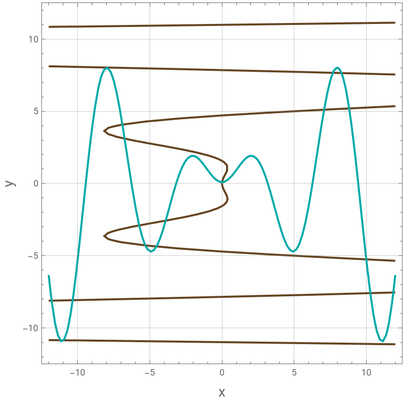
Consider the system of nonlinear algebraic equations:(x,y)=x-cos(y)=0 and (x,y)=-y+xsin(x)+=0, where =0.7 and =0.1.
This notebook finds all roots of this system in the domain.
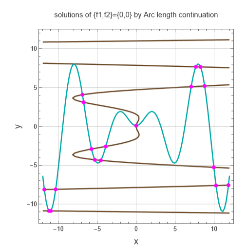
Method 1 uses Seader’s approach[1] and the arc length continuation technique.
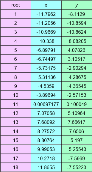
The problem considered is described as follows: (the function was first proposed in[1]), (x(s),y(s))=0, and ++=1 (i.e., the auxiliary equation). Using the built-in Mathematica function WhenEvent all roots of the system are readily obtained when . A list of all roots is provided.
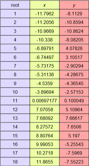
Method 2 uses a Particle Swarm Optimizer (PSO) to minimize the sum of squares ||f1(x,y)||^2+||f2(x,y)||^2 over the search domain. Because a root of the system is a global minimum (equal to zero) of this objective, and because the objective generally has many separate local minima corresponding to the different roots, the swarm is re-run from many independent random initializations; each run that converges to (near) zero loss yields one candidate root, and the collected candidates are filtered down to the list of distinct real roots.
Method 3 is based on Wagon’s work [2]. The zero-level curve of f1(x,y) is traced with ContourPlot, and the underlying polygonal line data (the Line primitives that Mathematica uses internally to draw the contour) is extracted directly from the resulting Graphics object with Cases. These points are then mapped through f2(x,y), and the loci where f2(x,y) changes sign along the f1=0 curve are located. Each such sign-change location is used as a starting guess, and FindRoot is applied there to pin down all the known 18 roots of the system in the domain [-12,12]×[-12,12].
Reference:
[1] S. K. Rahimian, F. Jalali, J. D. Seader, and R. E. White, “A New Homotopy for Seeking all Real Roots of a Nonlinear Equation,” Computers and Chemical Engineering, 35(3), 2011 pp. 403–411. doi:10.1016/j.compchemeng.2010.04.007
[2] S. Wagon, Mathematica® in Action: Problem Solving through Visualization and Computation, 3rd ed., Berlin: Springer-Verlag, 2010.
Consider the system of nonlinear algebraic equations:
f
1
2
y
z
1
f
2
z
2
z
1
z
2
This notebook finds all roots of this system in the domain
[-12,12]×[-12,12]
Method 1 uses Seader’s approach[1] and the arc length continuation technique.
The problem considered is described as follows:
H(t(s),x(s),y(s))=1-t(s)+(x(s),y(s))=0
f
1
H(t,x,y)
f
2
2
(t'(s))
2
(x'(s))
2
(y'(s))
t(s)=1
Method 2 uses a Particle Swarm Optimizer (PSO) to minimize the sum of squares ||f1(x,y)||^2+||f2(x,y)||^2 over the search domain. Because a root of the system is a global minimum (equal to zero) of this objective, and because the objective generally has many separate local minima corresponding to the different roots, the swarm is re-run from many independent random initializations; each run that converges to (near) zero loss yields one candidate root, and the collected candidates are filtered down to the list of distinct real roots.
Method 3 is based on Wagon’s work [2]. The zero-level curve of f1(x,y) is traced with ContourPlot, and the underlying polygonal line data (the Line primitives that Mathematica uses internally to draw the contour) is extracted directly from the resulting Graphics object with Cases. These points are then mapped through f2(x,y), and the loci where f2(x,y) changes sign along the f1=0 curve are located. Each such sign-change location is used as a starting guess, and FindRoot is applied there to pin down all the known 18 roots of the system in the domain [-12,12]×[-12,12].
Reference:
[1] S. K. Rahimian, F. Jalali, J. D. Seader, and R. E. White, “A New Homotopy for Seeking all Real Roots of a Nonlinear Equation,” Computers and Chemical Engineering, 35(3), 2011 pp. 403–411. doi:10.1016/j.compchemeng.2010.04.007
[2] S. Wagon, Mathematica® in Action: Problem Solving through Visualization and Computation, 3rd ed., Berlin: Springer-Verlag, 2010.
In[]:=
f1[x_,y_,z1_]:=x-Cos[y]z1;f2[x_,y_,z2_]:=-y+xSin[x]+z2;
2
y
In[]:=
z1=0.7;z2=0.1;
In[]:=
plt1=Show[ContourPlot[f1[x,y,z1],{x,-12,12},{y,-12,12},Contours{0},GridLinesAutomatic,ContourShading->False,ContourStyle{Thick,Darker@Brown},ImageSize.9{450,450}],ContourPlot[f2[x,y,z2],{x,-12,12},{y,-12,12},Contours{0},GridLinesAutomatic,ContourShading->False,ContourStyle{Thick,Darker@Cyan},ImageSize.9{450,450}],FrameLabel->{Style["x",14],Style["y",14]}]
Out[]=
Method 1
In[]:=
eq1=1-t+f1[x,y,z1]0/.tt[s]/.xx[s]/.yy[s];eq2=f2[x,y,z2]0/.tt[s]/.xx[s]/.yy[s];eq3=t'[s]^21-x'[s]^2-y'[s]^2;
In[]:=
init1=t[0]1.00000001;init2=x[0](x/.FindRoot[{f1[x,y,z1]0,f2[x,y,z2]0},{x,10.0},{y,-5.0},MaxIterations1000]);init3=y[0](y/.FindRoot[{f1[x,y,z1]0,f2[x,y,z2]0},{x,10.0},{y,-5.0},MaxIterations1000]);
In[]:=
{sol,pts}=Quiet@Reap@NDSolve[{eq1,eq2,eq3,init1,init2,init3,[0]-1,[0]0.025,y'[0]0.025,WhenEvent[t[s]1,Sow[{x[s],y[s]}]]},{t[s],x[s],y[s]},{s,-110000,1×10000}];
′
t
′
x
In[]:=
tbl=Sort@Select[Flatten[pts,1],12≥#[[1]]≥-12&];
In[]:=
Show[plt1,Epilog{Magenta,PointSize[0.02],Table[Point[{tbl[[i]][[1]],tbl[[i]][[2]]}],{i,1,Length[tbl]}]},PlotLabel->"\n solutions of {f1,f2}={0,0} by Arc length continuation \n"]
Out[]=
In[]:=
Text@Grid[Join[{{"root",Style["x",Italic],Style["y",Italic]}},Table[{i,tbl[[i]][[1]],tbl[[i]][[2]]},{i,1,Length[tbl]}]],Frame->All,ItemSize->{{7,7,7},Table[1.5,{i,1,Length[tbl]+1}]},Background->{{Hue[8/10,0.2,1],Hue[5/10,0.35,1],Hue[4/10,0.35,1]}}]
Out[]=
Method 2
In[]:=
(*ParticleSwarmOptimizer*)clipMatrix[mat_,lbv_,ubv_]:=Transpose[MapThread[Clip[#1,{#2,#3}]&,{Transpose[mat],lbv,ubv}]];clampMatrix[mat_,vmaxv_]:=Transpose[MapThread[Clip[#1,{-#2,#2}]&,{Transpose[mat],vmaxv}]];
In[]:=
psoOptimize[lossFunc_,dim_,lb_,ub_,nParticles_:30,nIter_:100,wMax_:0.9,wMin_:0.4,c1_:1.42,c2_:1.42,vClampFrac_:0.2,seed_:1]:=Module[{particles,velocities,pbest,pbestScore,gbest,gbestScore,convergence={},r1,r2,scores,gbestIdx,vmax,wIter},SeedRandom[seed];vmax=vClampFrac*(ub-lb);particles=Transpose@Table[RandomReal[{lb[[i]],ub[[i]]},nParticles],{i,dim}];velocities=ConstantArray[0.,{nParticles,dim}];pbest=particles;pbestScore=lossFunc/@particles;gbestIdx=First@Ordering[pbestScore,1];gbestScore=pbestScore[[gbestIdx]];gbest=pbest[[gbestIdx]];Do[wIter=wMax-(wMax-wMin)*(j-1)/(nIter-1);r1=RandomReal[1,{nParticles,dim}];r2=RandomReal[1,{nParticles,dim}];velocities=wIter*velocities+c1*r1*(pbest-particles)+c2*r2*(ConstantArray[gbest,nParticles]-particles);velocities=clampMatrix[velocities,vmax];particles+=velocities;particles=clipMatrix[particles,lb,ub];scores=lossFunc/@particles;pbest=MapThread[If[#3<#2,#1,#4]&,{particles,pbestScore,scores,pbest}];pbestScore=MapThread[Min,{pbestScore,scores}];gbestIdx=First@Ordering[pbestScore,1];If[pbestScore[[gbestIdx]]<gbestScore,gbestScore=pbestScore[[gbestIdx]];gbest=pbest[[gbestIdx]];];AppendTo[convergence,gbestScore],{j,nIter}];{gbest,gbestScore}];
In[]:=
(*ObjectivePSOwillminimize:squarednormofthegradient*)loss[{x_,y_}]:=f1[x,y,z1]^2+f2[x,y,z2]^2;
In[]:=
(*Runseveralindependentswarms(differentrandomseeds)sowe'relikelytolandonallcriticalpoints-maytakefewminutes*)results=Table[psoOptimize[loss,2,-14{1,1},14{1,1},30,100,0.9,0.4,1.42,1.42,0.2,seed],{seed,1,10000}];
In[]:=
tol=10^-1;cleaned=First[MinimalBy[#,Last]]&/@GatherBy[results,Round[#[[1]],tol]&];
In[]:=
final=Select[cleaned,Last[#]<=10^-8&];
In[]:=
final2=Table[final[[i]][[1]],{i,1,Length@final}];
In[]:=
tbl2=Sort@Select[final2,12≥#[[1]]≥-12&];
In[]:=
Length@tbl2
Out[]=
18
In[]:=
Text@Grid[Join[{{"root",Style["x",Italic],Style["y",Italic]}},Table[{i,tbl2[[i]][[1]],tbl2[[i]][[2]]},{i,1,Length[tbl2]}]],Frame->All,ItemSize->{{7,7,7},Table[1.5,{i,1,Length[tbl2]+1}]},Background->{{Hue[7/10,0.15,1],Hue[2/10,0.35,1],Hue[10/10,0.35,1]}}]
Out[]=
Method 3