An Improved Shooting Method Applied to the Blasius Problem
Authors: Housam Binous and Ahmed Bellagi
An Improved Shooting Method Applied to the Blasius Problem
Authors: Housam Binous and Ahmed Bellagi
Authors: Housam Binous and Ahmed Bellagi
We propose a new way to solve split boundary value problems using the shooting technique.
The new approach is based on NDSolve`StateData and is more than two times faster than the previous approach based on the work of Professor Brian Higgins, U C Davis.
The two approaches are successfully applied to solve the Blasius problem.
The new approach is based on NDSolve`StateData and is more than two times faster than the previous approach based on the work of Professor Brian Higgins, U C Davis.
The two approaches are successfully applied to solve the Blasius problem.
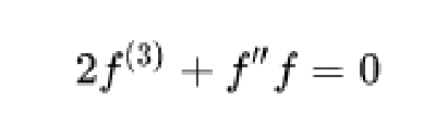
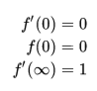
TheBlasiusequationisgivenby:withthefollowingboundaryconditions:Furtherinformationaboutthisproblemcouldbefoundhere:https://en.wikipedia.org/wiki/Blasius_boundary_layer
TheBlasiusequationisgivenby:
withthefollowingboundaryconditions:
Furtherinformationaboutthisproblemcouldbefoundhere:https://en.wikipedia.org/wiki/Blasius_boundary_layer
References :
1 - Blasius, H.(1908)."Grenzschichten in Flüssigkeiten mit kleiner Reibung".Z.Angew.Math.Phys.56 : 1–37.
2 - W.M.Deen, Analysis of Transport Phenomena, New York : Oxford University Press, 1998.
1 - Blasius, H.(1908)."Grenzschichten in Flüssigkeiten mit kleiner Reibung".Z.Angew.Math.Phys.56 : 1–37.
2 - W.M.Deen, Analysis of Transport Phenomena, New York : Oxford University Press, 1998.
Classic Approach of Professor Brian Higgins, U C Davis
Also, one can safely consider that η = 7 is equivalent to η = ∞ .
Also, one can safely consider that η = 7 is equivalent to η = ∞ .
In[]:=
MyODE[ξ_]:=NDSolve[{D[f[η],{η,3}]-1/2f[η]f''[η],f[0]0,f'[0]0,f''[0]ξ},f[η],{η,0,7}]bc[ξ_?NumericQ]:=First[D[f[η]/.MyODE[ξ],{η,1}]/.η7]FindRoot[bc[ξ]1,{ξ,0.001}]//Timing
Out[]=
{0.109201,{ξ0.332096}}
In[]:=
D[f[η]/.MyODE[0.33209637030937`],{η,1}]
Out[]=
InterpolatingFunction[η]


In[]:=
Plot[%,{η,0,7},PlotRangeAll,PlotStyleDarker@Red,FrameTrue,GridLinesAutomatic,AspectRatio1,ImageSize400{1,1},FrameLabel{Style["η",14],Style["f'[η]",14]}]
Out[]=
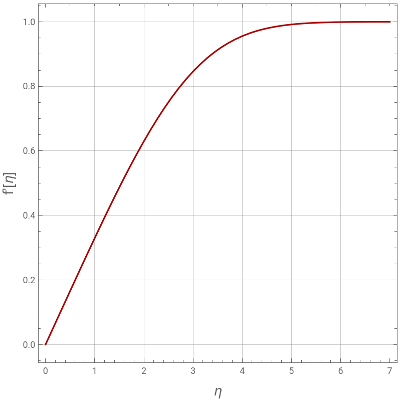
Checking our results: do we have
f'(∞)=1
In[]:=
D[f[η]/.MyODE[0.33209637030937`],{η,1}]/.η7//First
Out[]=
1.
Our new Approach is, depending on computer you are using, more than two times faster.
Using NDSolve`Reinitialize economises computational time. Indeed, one needs to solve the same differential equation for many different initial conditions in the shooting method for boundary value problems.
Again, one can safely consider that η = 7 is equivalent to η = ∞ .
Using NDSolve`Reinitialize economises computational time. Indeed, one needs to solve the same differential equation for many different initial conditions in the shooting method for boundary value problems.
Again, one can safely consider that η = 7 is equivalent to η = ∞ .
In[]:=
state=First[NDSolve`ProcessEquations[{D[f[η],{η,3}]-1/2f[η]f''[η],f[0]0,f'[0]0,f''[0]0.1},f[η],η]];newstate[ξ_]:=Module[{state1,sol1},state1=First[NDSolve`Reinitialize[state,{f[0]0,f'[0]0,f''[0]ξ}]];NDSolve`Iterate[state1,7];sol=NDSolve`ProcessSolutions[state1]]bc[ξ_?NumericQ]:=D[f[η]/.newstate[ξ],{η,1}]/.η7FindRoot[bc[ξ]1,{ξ,0.2}]//Timing
Out[]=
{0.0312002,{ξ0.332096}}
In[]:=
D[f[η]/.newstate[0.33209637030937`],{η,1}]
Out[]=
InterpolatingFunction[η]
In[]:=
Plot[%,{η,0,7},PlotRangeAll,PlotStyleDarker@Blue,FrameTrue,GridLinesAutomatic,AspectRatio1,ImageSize400{1,1},FrameLabel{Style["η",14],Style["f'[η]",14]}]
Out[]=
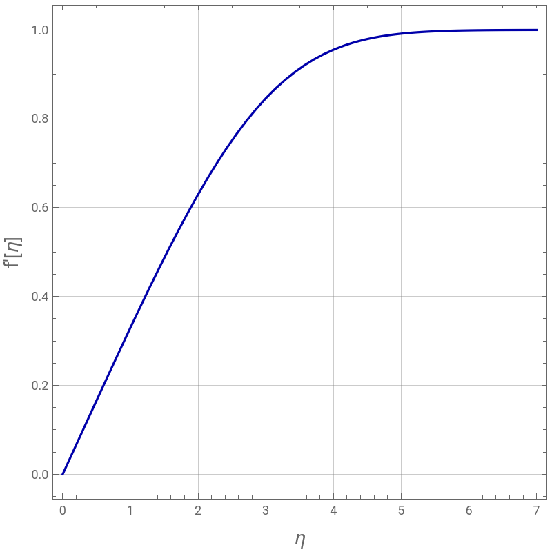
Checking our results: do we have
f'(∞)=1
In[]:=
D[f[η]/.newstate[0.33209637030937`],{η,1}]/.η7
Out[]=
1.