Residence Time Distribution Curve for the Tanks-in-Series Model
Authors: Housam Binous and Ahmed Bellagi
Authors: Housam Binous and Ahmed Bellagi
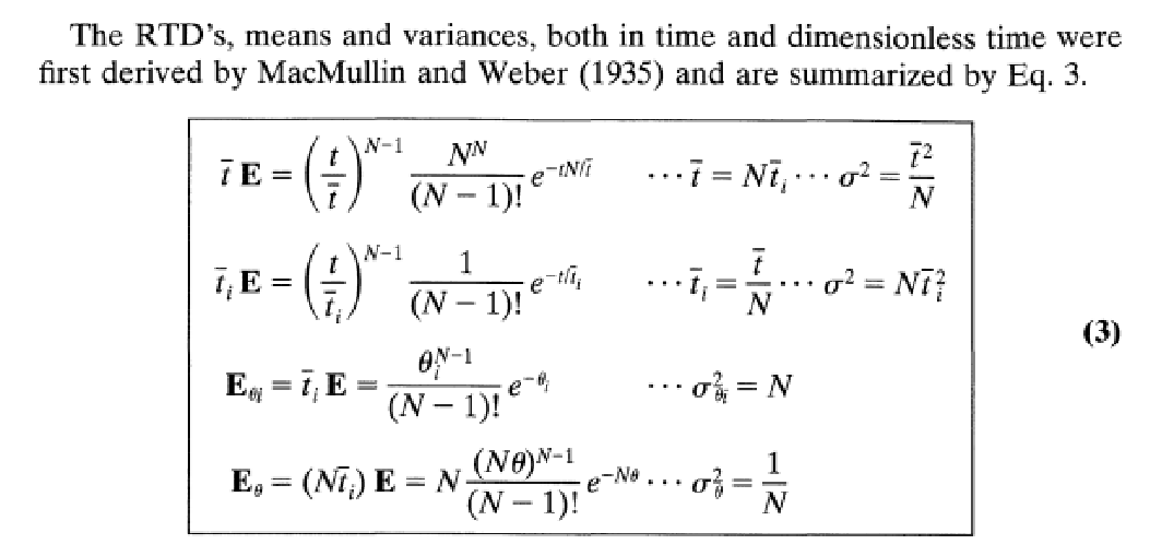
Expression of the Residence Time Distribution (RTD) for the tanks-in -series model were derived by MacMullin and Weber (1935) (see Ref. 1-2).
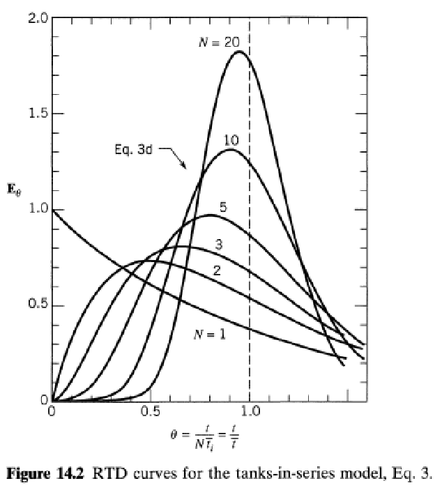
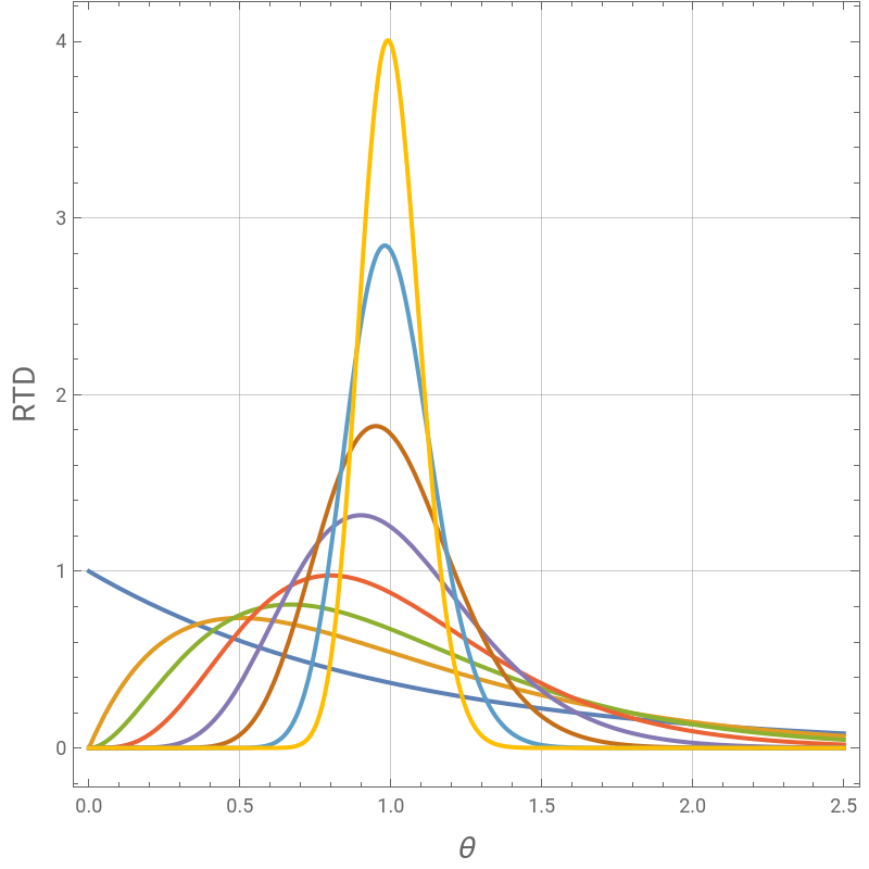
Here, we plot the RTD for a number of tanks equal to 1, 2, 3, 5, 10, 20, 50 and 100.
RTD is also computed from tracer pulse input for a number of tanks equal to 2, 5 and 50. In such case, the RTD is the outlet tracer concentration versus time curve. As expected both methods yield the same results.
Finally, for a particular tracer inlet function, we compute the outlet tracer concentration firstly by direct integration of the system of ordinary differential equations and secondly by application of the convolution theorem and the impulse response.
References:
1- O. Levenspiel, Chemical Reaction Engineering, 3rd Edition, Wiley, 1999, pages 323.
2- R.B. MacMullin and M. Weber, The Theory of Short-Circuiting in Continuous-Flow Mixing Vessels in Series and Kinetics of Chemical Reactions in Such Systems. Trans. AIChE. 1935; 31(2):409–458.
Expression of the Residence Time Distribution for the tanks-in-series model were first derived by MacMullin and Weber (Ref. 1-2). Here, we plot represents the RTD for a number of tanks i=1, 2, 3, 5, 10, 20, 50 and 100 tanks. θ is a dimensionless time.
In[]:=
ERTD[i_,θ_]:=i(iθ)^(i-1)/(i-1)!Exp[-iθ]
In[]:=
Quiet@Plot[{ERTD[1,θ],ERTD[2,θ],ERTD[3,θ],ERTD[5,θ],ERTD[10,θ],ERTD[20,θ],ERTD[50,θ],ERTD[100,θ]},{θ,0,2.5},PlotStyleThick,PlotRangeAll,AspectRatio1,GridLinesAutomatic,FrameTrue,FrameLabel{Style["θ",14],Style["RTD",14]},ImageSize400{1,1}]
Out[]=
RTD computed form tracer pulse input. RTD is the outlet tracer concentration versus time curve.
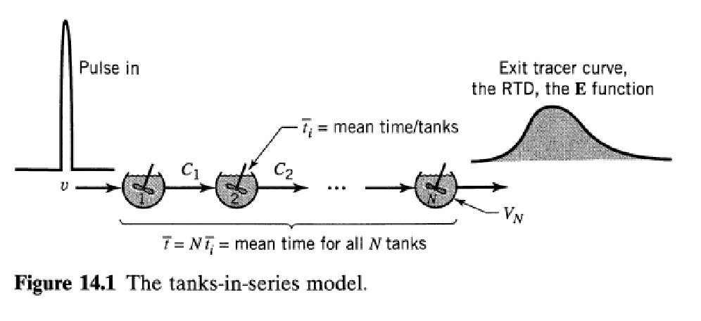
Tracer pulse input
In[]:=
CA
0
In[]:=
ϵ=1000000;
In[]:=
Plot[[t],{t,0,10/ϵ},PlotStyle{Thick,Darker@Red},PlotRangeAll,AspectRatio1,GridLinesAutomatic,FrameTrue,FrameLabel{Style["time",14],Style["tracer pluse",14]},ImageSize400{1,1}]
CA
0
Out[]=
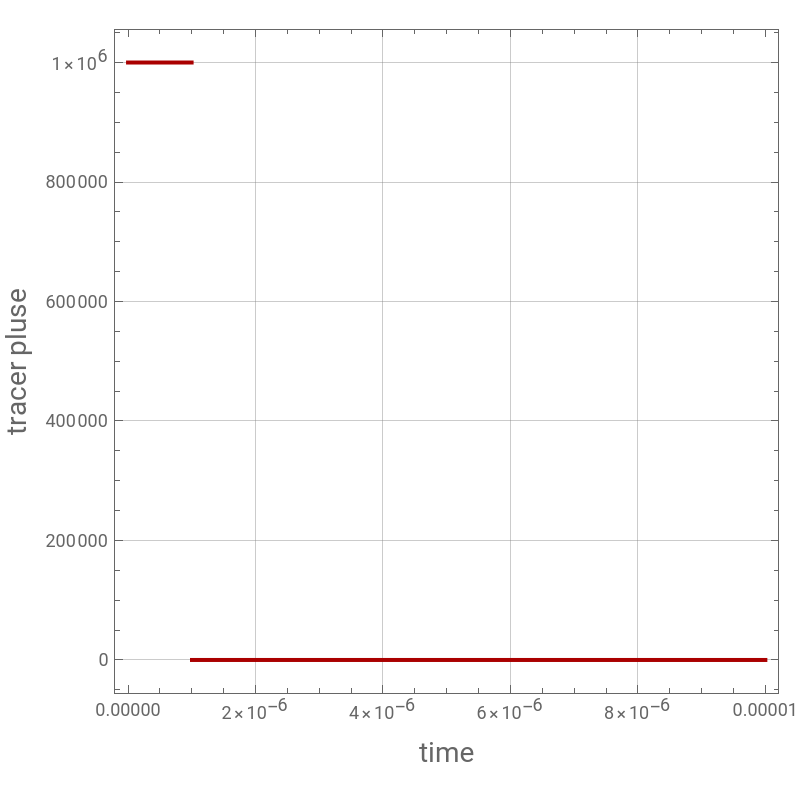
Mean residence time in a tank is τ. V is the total volume of all tanks. F is the flow rate and we consider a number of tanks equal 50.
Mean residence time in a tank is τ. V is the total volume of all tanks. F is the flow rate and we consider a number of tanks equal 50.
In[]:=
V=1; F=0.01; Ntanks = 50;
In[]:=
τ=V/F/Ntanks
Out[]=
2.
Governing Equations
In[]:=
i=2;
In[]:=
For[j=2,j<Ntanks+1,{eq[i]=D[[t],{t,1}]([t]-[t])/τ,i=i+1},j++]
CA
i
CA
i-1
CA
i
In[]:=
eq[1]=D[[t],{t,1}]([t]-[t])/τ;
CA
1
CA
0
CA
1
In[]:=
eqn=Table[eq[i],{i,2,Ntanks}];
In[]:=
Eq=Join[{eq[1]},eqn];
In[]:=
init=Table[[0]0,{i,1,Ntanks}];
CA
i
In[]:=
sys=Join[Eq,init];
In[]:=
Unknown=Table[,{i,1,Ntanks}];
CA
i
computing the exit concentration from each tank.
In[]:=
sol=NDSolve[sys,Unknown,{t,0,1000}];
Plot of the RTD using the concentration profile
In[]:=
plt1=Plot[[t]/.sol,{t,0,500},PlotStyleRGBColor[0,1,0],PlotRangeAll,AspectRatio1,GridLinesAutomatic,FrameTrue,FrameLabel{Style["time",14],Style["RTD",14]},ImageSize400{1,1}]
CA
50
Out[]=
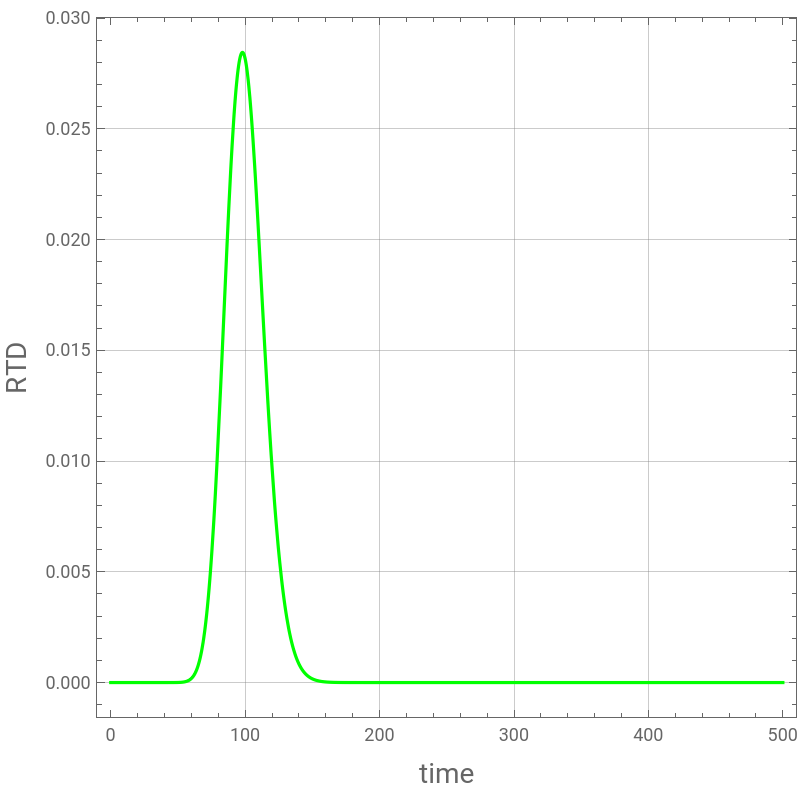
RTD from MacMullin and Weber's derivation (Ref. 1-2) for the 50 tanks case.
In[]:=
tbar=50 τ
In[]:=
RTD[t_]:=1/tbar (t/tbar)^(49) 50^50/49! Exp[-50 t/tbar]
Comparing the two methods of computation of the RTD
In[]:=
Show[plt1,plt2]
Mean residence time in a tank is τ. V is the total volume of all tanks. F is the flow rate and we consider a number of tanks equal 5.
Mean residence time in a tank is τ. V is the total volume of all tanks. F is the flow rate and we consider a number of tanks equal 5.
In[]:=
V=1; F=0.01; Ntanks = 5;
Governing Equations
In[]:=
i=2;
In[]:=
eqn=Table[eq[i],{i,2,Ntanks}];
In[]:=
Eq=Join[{eq[1]},eqn];
In[]:=
sys=Join[Eq,init];
computing the exit concentration from each tank.
In[]:=
sol5=NDSolve[sys,Unknown,{t,0,1000}];
Plot of the RTD using the concentration profile
RTD from MacMullin and Weber's derivation (Ref. 1-2) for the 5 tanks case.
In[]:=
tbar=5 τ
In[]:=
RTD[t_]:=1/tbar (t/tbar)^(4) 5^5/4! Exp[-5 t/tbar]
Comparing the two methods of computation of the RTD
In[]:=
Show[plt1,plt2]
Mean residence time in a tank is τ. V is the total volume of all tanks. F is the flow rate and we consider a number of tanks equal 2.
Mean residence time in a tank is τ. V is the total volume of all tanks. F is the flow rate and we consider a number of tanks equal 2.
In[]:=
V=1; F=0.01; Ntanks = 2;
Governing Equations
In[]:=
i=2;
In[]:=
eqn=Table[eq[i],{i,2,Ntanks}];
In[]:=
Eq=Join[{eq[1]},eqn];
In[]:=
sys=Join[Eq,init];
computing the exit concentration from each tank.
In[]:=
sol=NDSolve[sys,Unknown,{t,0,1000}];
Plot of the RTD using the concentration profile
RTD from MacMullin and Weber's derivation (Ref. 1-2) for the 2 tanks case.
In[]:=
tbar=2 τ
In[]:=
RTD[t_]:=1/tbar (t/tbar)^(1) 2^2/1! Exp[-2 t/tbar]
Comparing the two methods of computation of the RTD
In[]:=
Show[plt1,plt2]
If tracer inlet is now constant equal to 1 except between t = β and t = 2 β where it drops to zero.
Mean residence time in a tank is τ. V is the total volume of all tanks. F is the flow rate and we consider a number of tanks equal 5.
Mean residence time in a tank is τ. V is the total volume of all tanks. F is the flow rate and we consider a number of tanks equal 5.
In[]:=
V=1; F=0.01; Ntanks = 5;
Governing Equations
In[]:=
i=2;
In[]:=
eqn=Table[eq[i],{i,2,Ntanks}];
In[]:=
Eq=Join[{eq[1]},eqn];
In[]:=
sys=Join[Eq,init];
computing the exit concentration from each tank.
In[]:=
sol=NDSolve[sys,Unknown,{t,0,1000}];
Plot of the RTD using the concentration profile
RTD from MacMullin and Weber's derivation (Ref. 1-2) for the 5 tanks case.
In[]:=
V=1; F=0.01; Ntanks = 5;
In[]:=
RTD5[t_]:=1/tbar (t/tbar)^(4) 5^5/4! Exp[-5 t/tbar]
Obtaining the same dynamic response using the convolution theorem and the impulse response (i.e., RTD found above).
The solution obtained using the convolution theorem is represented with green dots.
The solution obtained using the convolution theorem is represented with green dots.
In[]:=
Off[NIntegrate::slwcon]
In[]:=
Off[NIntegrate::ncvb]
In[]:=
plt4=ListPlot[tblv1,PlotStyle{Darker@Green,PointSiez[0.02]},PlotRangeAll,AspectRatio1,
GridLinesAutomatic,FrameTrue,FrameLabel{Style["time",14],Style["tracer outlet concentration",14]},ImageSize400{1,1}]
GridLinesAutomatic,FrameTrue,FrameLabel{Style["time",14],Style["tracer outlet concentration",14]},ImageSize400{1,1}]
In[]:=
Show[plt1,plt4]