Wolfram Cloud Document

I decided to jump ahead one post because this worked out better than I expected. The attached notebook mentions conquering a dragon named Ansatz Schwarzschild, which really means deriving the Schwarzschild metric ab-initio in the UD calculus. I was going to post that notebook first, before this one, but it’s kind of dry: necessary physics and UD, but not necessarily entertaining. In the attached notebook, we conquer the much-more-fearsome dragon named Ansatz Kerr, with a magical sword named Ernst. The result is a beautiful Manipulate for exploring orbits around a spinning black hole. I promise to post about Ansatz Schwarzschild soon, but with that apology out of the way, here is the tale of the quest to conquer Ansatz Kerr.

Abstract

The Kerr metric around a spinning black hole is much more difficult than the Schwarzschild metric. The quest to find and solve its field equations took some 50 years from Einstein’s publishing of general relativity in 1915. The dramatis personae include Boyer, Lindquist, Kerr, Ernst, and others who published results from 1965 to 1968. We tell the story not historically, but as a fable of challenge and victory, in a spirit of rigorous fun. Along the way, we stress-test  and the Relativity Toolkit, v1.10.0. That’s the novel contribution of this notebook.

Unlike static Schwarzschild, Kerr has off-diagonal terms that couple time and rotation: frame-dragging. Light cones near the black hole are tipped in the spin direction, dragging orbits out of the Keplerian plane. The effect is also called gravitomagnetism, due to its resemblance to electrodynamical magnetism, both producing stresses perpendicular to planes of motion.

Over time, stable Kerr orbits trace out toroidal structures via nodal precession similar to that of a Lagrange top. This precession is additional to precession of the perihelion, present even in Schwarzschild (non-rotating) geometry. Kerr black holes also have Ergospheres, aka static limits, spacetime boundaries outside the event horizons. Inside an Ergosphere, spacetime itself flows faster than light. Inflowing geodesics are swept along the spinning direction of the black hole.

Introduction: A Quest

The Wizard Chandra reveals a quest: “I have an ancient artifact, a wondrous machine, more wondrous than Antikythera. I have partially translated its name: “Visualizer.” From what else I can gather, it shows orbits around a spinning black hole. I can make it do some things, but I can’t operate it proficiently. Find out anything you can about it. Needless to say, I also don’t know how it works. Is it beyond hope to find the blueprints? Without them, I can’t replicate, maintain, or repair the machine. If it breaks, it’s lost forever! Let me show you what little I know.”

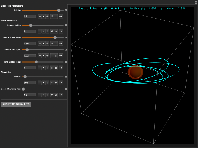
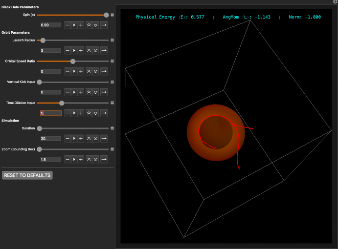
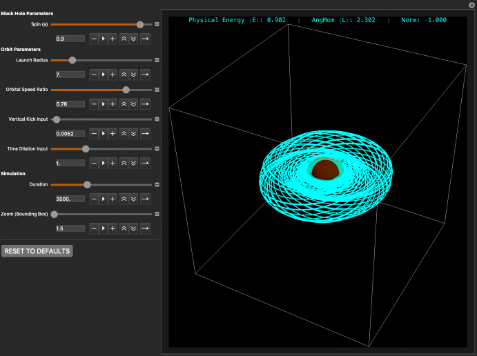
He shows us: The 3D Spirograph, wherein orbits fly up and down, out of the plane, but never escape a donut-shaped envelope; The Hula Hoop, wherein orbits become Schwarzschild—planar—when the black hole stops spinning; The Rip Tide, wherein stars dumped straight down into the black hole touch the Ergosphere and are swept aside and flung away.

We look inside the machine. The clockwork is an indecipherable bloc of definitions. Our quest is to explain them.

To do that, the wizard says, we must find, decipher, and translate the keys that lie in forgotten tomes in a Great Library fabled to be at the end of a long road. The wizard gives us a partial map, a linearized far-field approximation.

The wizard warns us that a dragon named Ansatz Kerr blocks the road. To look the ansatz field equations in the eye will drive a knight to madness. But, the wizard gives us pieces of a Magical Sword, Ernst, that he thinks might help us. These pieces are new compiler functions in the  Relativity Toolkit. We write down more of the wizard’s guide for our quest journey:

◼

The Dragon: We write the Einstein vacuum field equations,

Ricci=0

, over an ansatz metric of four diagonal components, as we did with Schwarzschild, but this time including a fifth, coupling term, conjured intuitively, in the two, symmetrical,

t—ϕ

slots.

◼

The Thorny Thicket: While the equations are easy for  to write, they are a stupendously large, thorny thicket of algebra on either side of the dragon, with 300-800 terms each. No opening has ever been found, the wizard tells us. There is no obvious structure amongst the enormity, no starting point for teasing the equations apart and solving them incrementally. (TODO: perhaps AI can take a stab at solving them; I didn’t try it.)

◼

The Wizard’s Map: Are we on the right road? The map is a new, simplified, linearized, weak-field, far-field ansatz that yields Newton-Kepler with light frame-dragging. The map will show us when we are on the right road, with the promise that the keys we seek lie beyond the dragon. But we can’t slay the dragon, and we can’t step around him because he is surrounded by the impenetrable thicket as far as the eye can see.

◼

The Magical Sword: a sword named Ernst may help us. If we can find the jewels in the thicket, we can slot them into the empty hilt of the sword and, by shining sunlight through them, enchant the monster into letting us pass. Ernst gives us a simplified equation that the Kerr metric must satisfy. The jewels will write the equation in  and recapitulate Ernst’s proof.

◼

The Road Beyond: Now with the full metric revealed, we compare it to the Wolfram Function Repository (WFR) and find a match. This will be the detailed map to the Great Library.

◼

The Quest Achieved: Should we succeed, we will find the vacuum equations now tractable, symbolically and numerically, and show how they’re built into the Visualizer. We now can explain, in detail, The 3D Spirograph, The Hula Hoop, The Rip Tide.

Before we set out, the wizard fully provisions us for the quest.

Basic Provisions: the Relativity Toolkit

Supplies for the journey ahead as we search for the keys to The Wondrous Machine.

Optional: Quit for a Fresh Kernel

◼

Note, if you call Quit in a notebook, evaluation may hang. If you want to “Evaluate Notebook,” mark the following two cells “Evaluatable” in the Cell

Property menu, call Quit and FrontEndTokenExecute once each, then comment out the cells, or mark them unevaluatable again. Alternatively, you can quit the kernel via the Evaluation menu (last item). At that point, you can “Evaluate Notebook” in a clean environment, or evaluate cells individually.

Quit[];

In[]:=

FrontEndTokenExecute["DeleteGeneratedCells"]

Download the Code

In[]:=

RTbranch="main";RTbase="https://raw.githubusercontent.com/rebcabin/RelativityToolkit/"<>RTbranch<>"/";RTbust="?t="<>ToString[Round[AbsoluteTime[]]];(*Forcefreshdownload*)RTrules=RTbase<>"RelativityToolkit.wl"<>RTbust;RTtests=RTbase<>"RelativityToolkit_RegressionTests.wl"<>RTbust;RTviz=RTbase<>"RelativityToolkit_VisualShowcase.wl"<>RTbust;Get[RTrules];

Relativity Toolkit version :1.10.0

Relativity Connection Symbol :Γ

Provisions for the Magical Sword: New Compiler Functions

The Wizard Chandra gave us the pieces for Ernst, The Magical Sword. We are sure we will need it, but we should not assemble it too early, lest we damage it. Furthermore, there is little point, as its magic requires the lost jewels we must find before anything else to enchant the dragon.

We add several new general-purpose functions to the  compiler corpus. This section sketches their functionality, and the rest of the notebook illustrates their use by example. These functions pertain to future problems in general relativity and differential geometry.

In this notebook, “matrix” is a synonym for a Wolfram 2D array. A tensor is either a matrix that satisfies coordinate-transformation rules, or a collection of symbolic  expressions that also satisfy coordinate-transformation rules.

A Summoning Spell: Γ-getter

Just as CalculateRicciComponent, already in the toolkit, needs a Riemann-getter for fetching components from Riemann, so CalculateRiemannComponent needs a Γ-getter for fetching components of the Christoffel symbols. Heretofore, Γ-getters were ad-hoc, constructed on-the-fly. But now we offer a way to build them from rule-patterned ancestors: the metric and its inverse.

Given symbols and rules for the covariant metric,

μν

, and its contravariant inverse,

μν

, CalculateGammaComponent is a general way to fetch an individual component at indices

[s]

[m]

[n]

of the Christoffel symbols. This definition and implementation mirrors its partners, CalculateRiemannComponent and CalculateRicciComponent, introduced in v1.9.0.

◼

The covariant and contravariant metrics stand in a mutually matrix-inverse relationship because

μρ

ρn

, the Kronecker delta, aka the Identity matrix.

In[]:=

CalculateGammaComponent[s_,m_,n_,gDD_Symbol,gDDRules_,gInvUU_Symbol,gInvUURules_,coords_]:=(ContractAll[ChristoffelsFromMetric[gDD,gInvUU,s,m,n],coords]/.gDDRules/.gInvUURules)//EvaluateUDPartials;

The Handguard: Gradient

For Ernst’s Equation (the Magical Sword), we’ll need the gradient operator in curved spacetime.

◼

It is also the workhorse of Hamilton-Jacobi Theory, whence we get the geodesic equations, e.g.

Because GradRaised needs only the contravariant metric, it takes only a symbol and rules for that.

The Hilt: Gradient Squared

The hilt of the Magical Sword, with the empty slots for the jewels, requires the squared gradient:

Like GradientRaised, GradSquared needs only the contravariant metric, taking only a symbol and rules for that.

The Blade: Scalar Laplacian

The blade of the Magical Sword is the Laplacian:

The Wondrous Machine: Kerr Orbit Visualizer

The wizard has translated part of a warning label on the Wondrous Machine: “this ancient artifact is designed to illustrate physically plausible scenarios. Given the particular decomposition of initial conditions and parameters, it is possible to create non-physical scenarios such as stars that travel faster than the speed of light. When this happens, a red light may appear in the Heads-Up Display.

Dependencies, Mute, En-Bloc

The quest should reveal the meaning of these definitions, but the wizard cannot translate them. For now, take them as granted, as just enough to enable the Visualizer.

Unknown functions of proper time τ

Explicit Acceleration Rules

The Visualizer itself

Kerr Visualizer User’s Manual

Along with the machine, the wizard has a priceless scroll, but he cannot translate it without the keys. We, however, as omniscient narrators of the tale, can read what the wizard and the adventurers cannot. Knowing it now, we will judge the success or failure of the quest.

Units

Fundamental Constants

For brevity, define

Examples

Angular momentum is measured in meters. The slider measures specific spin angular momentum of the black hole, normalized to the mass (in meters) of the black hole. Larger values mean faster spinning.

Example: The Sun

The Sun is a slow rotator. What if it were a black hole? What value should we put on the Spin slider?

The coefficient in the moment-of-inertia formula for a centrally condensed star like the Sun is about 0.070, much less than the 2/5 for a uniform sphere.

The starting distance of the test particle from the center of the black hole, aka the singularity at the center of the coordinate system.

◼

physical definition: Coordinate distance in Boyer-Lindquist coordinates.

Example: Sgr A*, supermassive black hole at center of the Milky Way

If we orbited Sgr A* at 1 AU, what should Launch Radius be?

An Independent Computation

Orbit SgrA* at a coordinate distance of 1 AU

Gravitational Radius of SgrA*

Launch Radius Slider Value

Time Dilation and the Heads-Up Display

Tip: If your particle flies off into space, i.e., becomes unbound, it has too much energy. Increase the time dilation to calm it down.

The calculators below let you predict what you should see in the HUD for various scenarios. Use them to verify your intuition and the physics of the simulation!

CALCULATOR 1: Relativistic Flyby, aka the Lorentz Factor

CALCULATOR 2: Stable Circular Orbit, aka Gravitational Time Dilation

Example: Interstellar Visitor

A probe flies by at 20% the speed of light.

Example: Parking Orbit

Example: Innermost Stable Orbit (ISCO)

Time is flowing 41% faster for us at a safe distance than for the astronaut in orbit.

Orbital Speed Ratio Slider

The “Orbital Speed Ratio” slider is calibrated to the Keplerian circular orbital speed for the chosen Launch Radius. The Visualizer does not accept independent settings for orbital radius and for orbital angular momentum, due to unusable sensitivity of such controls. Instead, the user specifies desired orbital angular momentum for a scenario as a ratio of desired speed to a Keplerian norm.

◼

Orbital angular momentum is the angular momentum of the test particle or star or spaceship orbiting the black hole, and is distinct from and independent of the spin parameter, which sets the angular momentum of the black hole itself.

Example: Earth’s Orbit Around the Sun

Not far from Wolfram-Alpha’s answer:



In[]:=

Earth's orbital speed around the Sun in km/s

In the Visualizer, setting Ratio to 1.0 achieves this balance automatically.

Example: Sgr A*, Supermassive Black Hole in the Milky Way

What’s the speed if we orbit Sgr A* at 1 AU’s distance? This is not for a slider setting, just for information.

2000 times the speed Earth needs around the Sun to keep from falling in.

Vertical Kick Input Slider, aka Inclination

The Vertical Kick slider imparts an initial velocity in the longitudinal θ direction, perpendicular to the equatorial plane. Physically, this creates orbital inclination or tilt.

### 4. Vertical Kick Input `initVelTheta` ($u^\theta$)

This is the initial velocity perpendicular to the equatorial plane.

With Schwarzschild (non-spinning) black holes, an inclined orbit is just a flat tilted ring. But with Kerr (spinning) black holes, frame dragging causes the entire orbital plane to precess.This creates the spirographical donut shapes you see in the Visualizer. The larger this kick,the "thicker" the donut.

This is the initial velocity perpendicular to the equatorial plane.

CALCULATOR: Kick to Inclination Angle (Approx)

This is a rough heuristic for the Visualizer’s behavior.

Example: Spirograph

This tilt lets the black hole’s spin twist the orbit into a torus.

Duration Slider

How long is'Duration=100' in human time?

Example: Duration 1000

The Wizard’s Experiments

Here are the settings that the Wizard knows. Neither he nor the adventurers know what they mean in any depth, but we, the omniscient narrators, are privileged to know now.

The 3D Spirograph (Toroidal Precession)

In the (+) mark upper right of the Manipulate box, choose the bookmark “The 3D Spirograph.” Alternatively, set parameters as follows

◼

Spin: 0.9 (default; high spin emphasizes the effect)

◼

Initial Radius: 7.0 (default)

◼

Orbital Speed Ratio: 0.78 (less than default)

◼

Vertical Kick: 0.0052 (less than default)

◼

Time Dilation: 1.0 (default)

◼

Duration: 3500 (try animating slowly (⊳) from duration 0 and 12-16 clicks on the down speed control)

◼

Bounding Box Scale: 1.5 (default)

In this bookmarked visualization, a particle traces a donut-shaped shell around the black hole. This is the Lense-Thirring Effect at moderate setting. The phenomenon changing the osculating plane is nodal precession.

The Result: With a non-rotating Schwarzschild black hole, this orbit would just be a precessing ellipse that stays on a single flat plane. But here, the black hole’s spin drags the entire space around with it, adding nodal precession.

As the particle orbits, the osculating plane (instantaneous plane of travel) is continuously twisted by the black hole’s spin. The nodes, where the orbit crosses the equator, circulate over time, causing the orbit to precess not just in the radial direction, like Mercury’s perihelion precession around the Sun, but in azimuth, painting a complex torus (donut) shape instead of just a ring. Near a spinning black hole, there is no such thing as a fixed orbital plane.

The Hula Hoop (Schwarzschild Limit)

In the (+) mark upper right of the Manipulate box, choose the bookmark “The Hula Hoop.” Alternatively, set parameters as follows

◼

Spin: 0.0 (the critical change)

◼

Initial Radius: 7.0 (default)

◼

Orbital Speed Ratio: 1.09 (change)

◼

Vertical Kick: 0.0078 (change)

◼

Time Dilation: 1 (change)

◼

Duration: 6000 (change)

◼

Bounding Box Scale: 4 (change)

The donut, and the apparent chaos, disappears. Try animating spin slowly (10 clicks on the down-speed control for spin).

The Rip Tide

In the (+) mark upper right of the Manipulate box, choose the bookmark “The Rip Tide.” Alternatively, set parameters as follows

◼

Spin: 0.99 (max)

◼

Initial Radius: 3 (change)

◼

Orbital Speed Ratio: 0 (change)

◼

Vertical Kick: 0 (change)

◼

Time Dilation: 1.0 (default)

◼

Duration: 30 (change)

◼

Bounding Box Scale: 1.5 (default)

In this bookmarked visualization, we have a situation where Newtonian intuition breaks down.

The Deadly Fate: The red trail does not fall straight in. Instead, it’s violently ripped around the black hole in a spiral before plunging in.

This illustrates the Lense-Thirring effect (frame-dragging) at its extreme.

Inside the orange shell—the Ergosphere—the spin of the black hole drags spacetime along with it so fast that space itself move at the speed of light relative to a distant observer.

The boundary of the Ergosphere is the static limit. Inside this boundary, it is impossible to remain “static,” at a constant longitude ϕ. To stand still here would require moving against the flow of space faster than light.

Even though the particle has zero angular momentum—it’s trying to fall straight in—any coordinate grid the particle lives on is rotating. The effect is intrinsic to the geometry. No non-singular coordinate system (gauge choice) can get rid of it. The particle is swept downstream by the rip tide of spacetime. It is forced to co-rotate with the black hole, no matter how hard it resists.

The Dragon: Kerr Metric ab-initio

The Wizard Chandra warned us: “Do not look the dragon, Ansatz Kerr, in the eye, for his gaze is madness.” But being brave (foolhardy?), we go straight into the breach. The elder dragon, Ansatz Schwarzschild, yielded to a frontal attack, after all. Why not Ansatz Kerr?

We have found the dragon, but we cannot slay it and cannot step through the thicket around him. The equations are too dense, too coupled, and too angry to yield a solution by force. We need a better plan. We need the Wizard’s Map and the Magical Sword.

Here is how we got the thicket in the first place—our first attempt at finding a metric for a spinning black hole:

◼

Set up ansatz for a stationary, axisymmetric metric.

◼

Sub-strategy: Calculate Ricci components from toolkit functions ChristoffelsFromMetric and CalculateRiemannComponent.

◼

Unlike Schwarzschild, find that the Ricci equations are unwieldy: it’s not at all clear how to drive Wolfram to produce a result.

◼

Symbolically demonstrate Newtonian gravitation and mild gravitomagnetism in the weak-field limit, when the orbiting star is far from the black hole.

◼

Follow a historical derivation of the full solution: the Ernst Equation.

Stationary Axisymmetric Ansatz

Rules for the  toolkit

Instead of sparse matrices, we prefer rules for the non-zero components for further processing.

Symbolic inverse

Append catch-all zero rules;

Ricci via the Toolkit

Toolkit function CalculateRicciComponent requires a Riemann-getter function. The Riemann-getter calls toolkit function CalculateRiemannComponent, which requires a Γ-getter function. Define that first.

Γ-getter

It’s only useful to show a smattering of these equations, so we apply Short to them.

The components of the Ricci tensor are large, unwieldy expressions. Though not challenging for Wolfram to write, we did not see how to get Wolfram to solve. It’s not instructive to print them out, but it is instructive to illustrate how big and unstructured they are, to make the point that we should not try to solve them directly, but find another way. We won’t be using the vacuumFieldEquations above in the following sections, which take a different approach.

It’s big

It’s complicated: not a lot of regularity.

Optional: take the semicolon off the end of this this cell if you want to see an overwhelming, large graph, which is NOT necessary to understand the rest of the story.

Riemann of the Ansatz

Here we see the leaf counts of the 88 non-zero components of the Kerr curvature tensor. Symmetries and antisymmetries are immediately visible.

The Wizard’s Roadmap: Linearized Weak-Field Gravity

We beat a close escape from the dragon’s fire to study the parchment Chandra slipped into our backpack. It is a map of the “Far Lands”—the weak-field limit beyond the dragon, where gravity is gentle and the dragon’s roar is but a whisper.

We linearize our new ansatz metric, stripping away higher-order terms. We are left with an easy equation. If we solve it, and it reveals a dipole, we know that despite the smoke and fire ahead of us, we are at least confronting the right beast blocking the right road.

Weak Metric

Linearize the Metric Inverse

Rules for the Toolkit

As usual, we prefer rules over matrices:

Join with zero rules, as before:

Linearized Vacuum Field Equation

Proceed as before.

Γ-Getter

Solution

QED■

The Magical Sword: Ernst Equation for Kerr

The map confirms we are on the right road, but the dragon, Ansatz Kerr, still blocks our passage. We cannot slay the dragon. There is nothing else to do but hack at the thicket. In there, the wizard told us, we will find the jewels to slot into the hilt of the Magical Sword, by which to enchant the dragon. But we should not hack with ordinary, dull blades. We will use the sword itself to hack the thicket!

Our faithful squire, the  Toolkit, fetches the parts: the Blade (the Scalar Laplacian), the handguard (the Gradient), and the Hilt (the Gradient Squared) with its empty slots. We have only to assemble them and start hacking. If we can strike true, the thicket will cough up the jewels.

We follow Ernst’s assembly papers closely, positing the metric, then showing it solves a physically equivalent equation. Space does not permit a full recapitulation of his papers, but references are included below.

The Einstein equations reduce to a single non-linear equation, as opposed to five, coupled, non-linear equations:

We now proceed to show that the Kerr metric satisfies this equation.

Convenience Forms

Metric Proposal

Rules

Gradient, ∇ℰ

Gradient Squared, ∇ℰ∇ℰ

Determinants

Needed for the covariant Laplacian

Covariant Laplacian

Ernst Potential

Split Re/Im Parts

Wrap Operators

QED■

We’ve shone sunlight through the jewels. The dragon staggers off the road, stunned and dazed.

The Road Beyond the Dragon: Comparing to the WFR

Now that we are past the dragon, the details of the Wizard’s Map become clear. We travel to the Great Library (the Wolfram Function Repository) to seek our prize. In the library, we shine sunlight through the jewels again, onto the pages of the forgotton tomes, and the user’s manual and blueprints are fully revealed in language we understand.

An image of the Magical Sword and its jewels, just as we have in hand, appears as well. We compare our sword to the image. It is a perfect match. The very jewels that enchanted the are the secret key to the Wondrous Machine! Our quest is over, and we thought we had only begun! The Visualizer is no longer an incomprehensible artifact. The Wondrous Machine is a solved and understood instrument, ready for us to explore the Ergosphere and beyond.

Retrieving the Kerr Metric from WFR

Just a new name for the metric defined above

QED■

The Quest Achieved: Vacuum Solution for Kerr

Confronting Ansatz Kerr head-on got us burnt by dragon’s fire and scarred by thorns in the thicket. Now, back at home, with the jewels inserted into a computer, we receive silent but joyous zeros.

Above, in Ernst Equation for Kerr, we already define rules for the Kerr metric and its inverse, the contravariant form. To review:

Γ-Getter

Check a non-zero component

Riemann Helper

Check All Components

If this vanishes, then Kerr is a vacuum solution.

QED■

Epilogue

We began this quest with a mysterious artifact : a Visualizer that produced beautiful, chaotic orbits but whose inner workings were a riddle .

The Wizard Chandra warned us that the machinery—the Kerr metric—was too complex to understand by force. He was right. Confronting the dragon (the ab-initio vacuum equations) earned us firethorns of algebra. But, we retreated only from the blaze, not from the quest. Consulting the Wizard' s Map (the linearized limit), we were sure that the keys lay ahead. We assembled the Magical Sword (the Ernst Equation) from provisions carried by our faithful squire, the  Toolkit. With that sword, we pierced the thicket and found the enchanting jewels to pacify the dragon. The terrifying complexity of the spinning black hole—the frame-dragging, the time dilation, the time-azimuth coupling—collapses into a single, elegant identity The Rip Tide of the Ergosphere is not a glitch, it is twisting spacetime. We showed that our faithful  squire is strong enough and that our tools are sharp enough for whatever monsters lie ahead.

References

Ernst, F. J., New Formulation of the Axially Symmetric Gravitational Field Problem. Physical Review, Vol. 167, No. 5, pp. 1175-1178 (1968). [DOI: 10.1103/physrev.167.1175]

Ernst, F. J., New Formulation of the Axially Symmetric Gravitational Field Problem. II. Physical Review, Vol. 168, No. 5, pp. 1415-1417 (1968). [DOI: 10.1103/physrev.168.1415]

Ernst, F. J., New Formulation of the Axially Symmetric Gravitational Field Problem. II [Erratum]. Physical Review, Vol. 172, No. 5, p. 1850 (1968). [DOI: 10.1103/physrev.172.1850.3]

Kerr, R. P., Gravitational Field of a Spinning Mass as an Example of Algebraically Special Metrics. Physical Review Letters, Vol. 11, No. 5, pp. 237-238 (1963). [DOI: 10.1103/PhysRevLett.11.237]

Boyer, R. H., Maximal Analytic Extension of the Kerr Metric. Journal of Mathematical Physics, Vol. 8, No. 2, pp. 265-281 (1967). [DOI: 10.1063/1.1705193]

Newman, E. T., Couch, E., Chinnapared, K., Exton, A., Prakash, A., & Torrence, R., Metric of a Rotating, Charged Mass. Journal of Mathematical Physics, Vol. 6, No. 6, pp. 918-919 (1965). [DOI: 10.1063/1.1704351]

Hartle, J. B., Gravity: An Introduction to Einstein's General Relativity. Benjamin Cummings (2003)."

Chandrasekhar, S., The Mathematical Theory of Black Holes. Oxford University Press (1983). Chapter 6, Section 53.

Beckman, Brian . From the steam age to quantum fields: a unified approach via UD tensorial calculus. Wolfram Community post.

Beckman, Brian . General relativity in the UD calculus. Wolfram Community post.

Beckman, Brian . Formal Differential Geometry in the UD Calculus: Part 1. Wolfram Community post.

Beckman, Brian. Covariant Derivatives and Connections in the  Calculus. Wolfram Community post.

Beckman, Brian. Riemann Curvature in  + Compiler POC. Wolfram Community post (to appear).

Beckman, Brian. Schwarzschild Orbits in the  Calculus. Wolfram Community post (to appear).

Beckman, Brian. Schwarzschild Metric from Scratch via  Compilation. Wolfram Community post (to appear).

Wolfram Function Repository . MetricTensor. For ground truth.

Wolfram Function Repository . ChristoffelSymbol. For ground truth.

[MTW] Misner, Charles W.; Thorne, Kip S.; Wheeler, John Archibald . Gravitation. Princeton University Press, 2017.

Petrov, A. Z. Classification of spaces defining gravitational fields, Scientific Transactions of Kazan State University, 114, 55 (1954)

CITE THIS NOTEBOOK

A wizard's quest: spinning black holes in 
by Brian Beckman
Wolfram Community, STAFF PICKS, February 8, 2026
https://community.wolfram.com/groups/-/m/t/3636508