Introduction
Introduction
Introductory courses in differential equations typically focus on real-valued solutions. Even in the eigenvalue-eigenvector method for autonomous linear ODEs, the real and imaginary parts of the complex-valued solutions, as real-valued functions, are taken to be the desired solutions. This is natural, since most of the students are from STEM fields in which most (but not all) of the applications of differential equations use real-valued solutions. This investigation into complex-valued solutions was prompted by a simple question in the current (4/2026) discussion for the Daily Study Group on differential equations.
Let be the standard representation of a complex number in terms of its real and imaginary parts. Let =+i denote the velocity vector of , where the components =,= are real-valued and is a real parameter. A differential equation of the form =f(t,z) is equivalent to a system of equations. Indeed, one can consider the ODE from the point of view of coupled systems: Suppose is a complex-valued function of a real variable and a complex variable . Then the system =(t,x,y),=(t,x,y) is equivalent to =f(t,z). An advantage of the complex form is the ability to investigate the interplay of the vector field of the differential equation with the connection between complex arithmetic and geometric transformations.
z=x+iy
dz
dt
v
x
v
y
z
v
x
dx
dt
v
y
dy
dt
t
dz
dt
f(t,x+iy)=(t,x,y)+i(t,x,y)
v
x
v
y
t
z=x+iy
dx
dt
v
x
dy
dt
v
y
dz
dt
In this note, our differential equation is autonomous, one of the form =f(z). In particular, the question that led to this note is what are the equilibria of =+1. There are no real ones, which was the given answer, but it prompted the question, can the imaginary number be an equilibrium? This leads to the notion of Apollonian circles, which are a solution to a geometry problem that we will introduce later.
dz
dt
dz
dt
2
z
i
Let’s first investigate the complex solutions to =+1, for the analysis of this equation will lead to question about its geometry.
dz
dt
2
z
The complex solutions
The complex solutions
The basic idea of a differential equation (ODE) in which the independent variable is a single real parameter is the same in both the real-valued and complex-valued settings: The rate of change of a variable, say , is given at each value of and time . New values are computed from one time to another by adding the rate times the change in time, in a similar way to the way that an integral is found via Riemann sums. In the limit as the changes in time are decreased, under suitable hypotheses on the rate function, the process converges to a solution. In the complex case, the increments to at each step add a complex number to the current value: =+v(,)Δ.
z
z
t
∫vdt
z
z
k+1
z
k
t
k
z
k
t
k
Here's a numerical illustration of the ODE =+1:
dz
dt
2
z
Block[{dz,dt,f},dt=0.1;(*time-stepsize*)f[z_]:=z^2+1;(*ODE:dz/dt=f[z]*)steps=NestList[Function[z,dz=f[z]dt;(*estimatedstep*)z+dz(*newvalueofz*)],0.3I,10];Legended[ComplexListPlot[steps,PlotHighlighting->None,PlotLabel->Row[{Row[{d,z}]/Row[{d,t}]," = ",f[z]}]],Grid[Prepend[steps,z]//Transpose@{#,f[#]}&,Alignment->"+",BaseStyle->{PrintPrecision->3}]]]
Out[]=
|
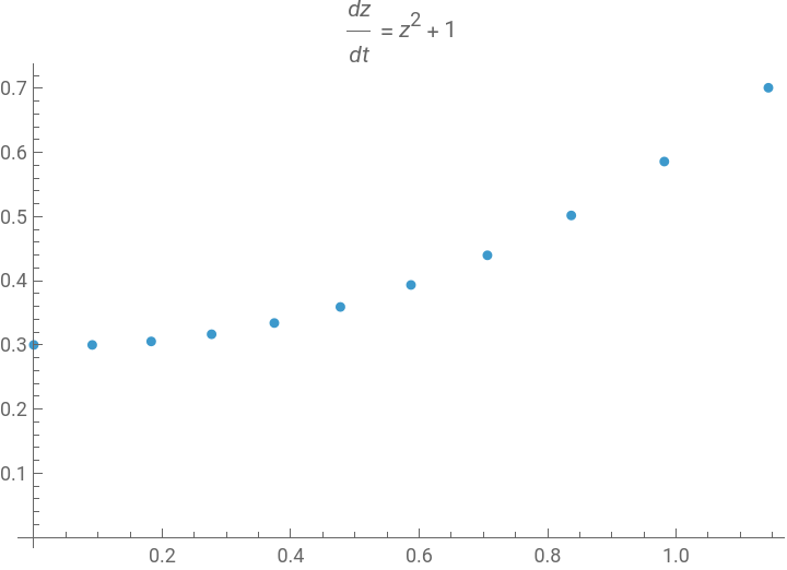
Here is another illustration using StreamPlot[] for a more complete picture of the stream lines (also called phase curves). The first line below shows how to obtain the vector field of the real coupled system associated to =+1. The corresponding system is
dz
dt
2
z
dx dt | = | 1+x^2-y^2 |
dy dt | = | 2xy |
vf=z^2+1/.z->x+I*y//ReIm//ComplexExpand
Out[]=
{1+-,2xy}
2
x
2
y
StreamPlot[vf,{x,-3,3},{y,-3,3},FrameLabel->{x,I*y}]
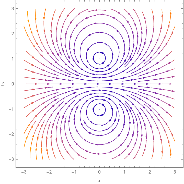
Cool. They look like circles. In fact, they remind me of Apollonian circles; see https://en.wikipedia.org/wiki/Apollonian_circles. And do appear to be equilibria.
±i
Apollonian circles
Apollonian circles
As a geometry problem
As a geometry problem
An Apollonian circle is the locus of a point , whose distances from two fixed points and form a constant ratio . In terms of complex numbers, the circle is represented by the following equation:
Z
A
B
r
Abs[Z-A]
Abs[Z-B]
If we choose and , we get a picture that is similar to the stream plot above. It turns out that it is easier to perform computations with the square of the ratio (Abs[Z-A]/Abs[Z-B])^2==r^2 instead directly with the ratio Abs[Z-A]/Abs[Z-B]==r.
A=i
B=-i
Block[{Z=x+I*y,Y,A=I,B=-I},apollonius=(Abs[Z-A]/Abs[Z-B])^2==r^2//ComplexExpand//Simplify]ContourPlot[Subtract@@apollonius/.r0,{x,-3,3},{y,-3,3},Contours(N@Range[-20,20]/5),ScalingFunctions"Log",FrameLabel{x,I*y}]
Out[]=
2
x
2
(-1+y)
2
x
2
(1+y)
2
r
Out[]=
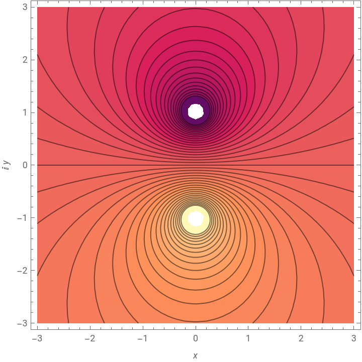
It turns out that the family of circles passing through the fixed points and intersect each of the Apollonian circles orthogonally (that is, their tangent lines at the point of intersection are perpendicular). Thus we have two families of circles, the first being the Apollonian circles varying with the parameter and the other being the orthogonal families. Both are sometimes called Apollonian circles. We will mainly discuss the first family, defined in terms of the ratio , but we will return to the second in the section on "Orthogonal trajectories of complex differential equations."
A
B
r
r
Below are some formulas we will use to analyze an Apollonian circle.
(*diametricalpointsQ=q*I,P=p*I*)diam=SolveValues[apollonius/.x->0,y](*centerC=c*I*)diam//Mean//Simplify(*p*q==1*)Times@@diam//Simplify(*lengthofdiameter*)diam[[2]]-diam[[1]]//Simplify
Out[]=
,
-1-r
-1+r
1-r
1+r
Out[]=
1+
2
r
1-
2
r
As a rate problem
As a rate problem
One way to obtain a solution:
From the geometry problem to the differential equation
From the geometry problem to the differential equation
We start from the Apollonian relation:
From the differential equation to the geometry problem
From the differential equation to the geometry problem
Symmetry of the ODE
Symmetry of the ODE
Therefore, we may, without loss of generality, restrict our attention to studying the differential equation in the upper half-plane.
Differential invariants
Differential invariants
To pique the reader's curiosity: Does a quick glance at the formulas suggest the solution curves are circles? The normal tangent has asymptotes, which I don't see in the stream plot. Maybe the complex tangent is more interesting? Sines and cosines are connected to circles, but the parametrization is not a simple, familiar form of a circle.
If one did not know the equation of the circle, or even whether the solution curve was a circle, one could test whether the curvature was constant, a differential invariant:
In this way we have constructed the solution to geometry problem:
Orthogonal trajectories of complex differential equations
Orthogonal trajectories of complex differential equations
In the code, {1,I}(z^2+1) ultimately evaluates to two vector fields. One is defined by z^2+1, the original differential equation, and the other is multiplied by I, that is, rotated 90º, which yields the orthogonal trajectories.
Bipolar coordinates
Bipolar coordinates
The mesh lines in a parametric plot show the two families of circles:
Check that it solves the initial value problem:
Exercises
Exercises
CITE THIS NOTEBOOK
CITE THIS NOTEBOOK
Apollonian circles and differential equations
by Michael Rogers
Wolfram Community, STAFF PICKS, April 22, 2026
https://community.wolfram.com/groups/-/m/t/3699888
by Michael Rogers
Wolfram Community, STAFF PICKS, April 22, 2026
https://community.wolfram.com/groups/-/m/t/3699888