Data Source
Data Source
The latest data gets updated on dashboard above before it is loaded to GitHub, which is the source for the notebook.
Procedures
Procedures
In[]:=
Clear[modelFitDisplay];modelFitDisplay[NLM_,data_,opts___]:=Module[{bands,p0,p1},bands[t_]=NLM["SinglePredictionBands",ConfidenceLevel0.95];p0=Plot[{NLM[t],bands[t]},{t,1,data[[-1]][[1]]+5},opts,Filling{2{1}},PlotStyle{Darker@Red,Darker@Orange,Darker@Orange},GridLinesAutomatic,PlotRangeAll,opts];p1=ListPlot[data,PlotRangeAll];Show[p0,p1]];
In[]:=
Clear[derivativeDisplay];derivativeDisplay[NLM_,data_,opts___]:=Module[{daynum,end,peak},daynum=data[[-1]][[1]];peak=t0/.NLM["BestFitParameters"];end=x/.FindRoot[NLM'[x]1,{x,peak,peak+200},(*forcetorighttail*)Method"Brent"][[1]];Print["Last case: ",DateString[DatePlus[{2020,1,21},Ceiling@end],"DateShort"]];Show[Plot[{NLM'[x],NLM''[x]},{x,data[[1]][[1]]-4,daynum+5},opts,GridLinesAutomatic,PlotRangeAll,PlotLegends{"First Derivative","Second Derivative"}],ListPlot[Tooltip[#,#]&/@{{daynum,NLM'[daynum]}},PlotStyle{Red,PointSize[0.02]}]]];
In[]:=
Clear[dataD1];dataD1[data_,{k_,L_}]:=Table[{data[[i]][[1]],kdata[[i]][[2]](1-data[[i]][[2]]/L)},{i,Length[data]}];
In[]:=
logistic=L/(1+Exp[-k(t-t0)]);
In[]:=
Clear[logisticDEFit];logisticDEFit[data_,k0_:0.3,L0_:2000,graphic_:True,optsInterpolation___]:=Module{dataFn,dataDE,dataDEPlot,deModel,deNLM,bands},dataFn=Interpolation[data,optsInterpolation,Method"Spline"];dataDE={dataFn[#],dataFn'[#]}&/@data[[All,1]];dataDEPlot=ListPlot[dataDE,PlotStyleDarker@Red,GridLinesAutomatic,PlotRangeAll];deModel=kx1-;deNLM=NonlinearModelFit[dataDE,{deModel,L>0},{{k,k0},{L,L0}},x];If[graphic,bands[L_]=deNLM["SinglePredictionBands",ConfidenceLevel0.95];Print@Show[Plot[{deNLM[x],bands[x]},{x,0,Abs@L/.deNLM@"BestFitParameters"},GridLinesAutomatic,Filling{2->{1}},FrameTrue,FrameLabel{"Cases","New Cases Per Day"},PlotRangeAll,PlotLabel"Logistic Differential Equation"],dataDEPlot]];Flatten@{deNLM@"BestFitParameters",FindRoot[dataFn[t0]L/2/.deNLM["BestFitParameters"],{t0,data[[-1]][[1]]}]};
x
L
Data Download
Data Download
In[]:=
confirmed=Import["https://raw.githubusercontent.com/CSSEGISandData/COVID-19/master/csse_covid_19_data/csse_covid_19_time_series/time_series_19-covid-Confirmed.csv"];confirmed[[1]][[-1]]confirmedData=AssociationThread[First@confirmed,#]&/@Rest[confirmed]//Dataset;keys=Keys[First@Normal@confirmedData];skoreaCaseData=confirmedData@Select[#"Country/Region""South Korea"&];skoreaCases0=Transpose[{Range[Length@keys-4],Values@Normal[skoreaCaseData[All,Drop[keys,4]]][[1]]}];
Out[]=
3/5/20
South Korea Case Correction
South Korea Case Correction
I suspect that the flat growth up to day 29 shows a small group of infected and exposed people successfully quarantined. Suddenly on day 30 there is a new outbreak, probably from an unknown source who wasn’t tracked with the initial group.
In[]:=
ListPlot[Tooltip/@skoreaCases0,PlotRangeAll]
Out[]=
In[]:=
skoreaNLM0=NonlinearModelFit[Take[skoreaCases0,29],logistic,{{k,0.3},{L,50},{t0,20}},t];skoreaNLM0@"BestFitParameters"
Out[]=
{k0.299198,L29.9925,t012.8662}
The first 29 days of the South Korea epidemic look like an epidemic which was essentially over. With the first cases successfully quarantined and isolated. The evidence of a new outbreak shows up on day 30.
In[]:=
modelFitDisplay[skoreaNLM0,Take[skoreaCases0,29],PlotLabel"Early South Korea Cases"]
Out[]=
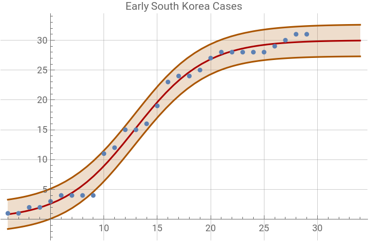
So we remove those 29 cases and subtract 30 from the accumulated data, to get the new epidemic.
In[]:=
skoreaCases={#1,#2-31}&@@@Drop[skoreaCases0,29]
Out[]=
{{30,73},{31,173},{32,402},{33,571},{34,802},{35,946},{36,1230},{37,1735},{38,2306},{39,3119},{40,3705},{41,4304},{42,5155},{43,5590},{44,6057}}
South Korea
South Korea
In[]:=
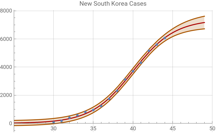
skoreaNLM=NonlinearModelFit[skoreaCases,logistic,{{k,0.3},{L,2000},{t0,50}},t];skoreaNLM["BestFitParameters"]modelFitDisplay[skoreaNLM,skoreaCases,PlotLabel"New South Korea Cases",PlotRange{{25,50},All}]
Out[]=
{k0.381513,L7392.43,t039.9908}
Out[]=
In[]:=
skoreaNLM@"ParameterConfidenceIntervalTable"
Out[]=
Estimate | Standard Error | Confidence Interval | |
k | 0.381513 | 0.0143124 | {0.350329,0.412697} |
L | 7392.43 | 236.802 | {6876.48,7908.37} |
t0 | 39.9908 | 0.211396 | {39.5302,40.4513} |
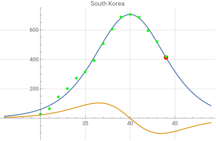
The graphic below shows the first and second derivative plots of the logistic function. The red dot is at the current day number on the first derivative curve. The green dots are the points calculated by the logistic differential equation, using each data point. The prediction for the last case date is printed (probably not accurate until there are at least three weeks of new data).
In[]:=
kdp1=derivativeDisplay[skoreaNLM,skoreaCases,PlotLabel"South Korea"];Show[kdp1,ListPlot[dataD1[skoreaCases,{k,L}/.skoreaNLM["BestFitParameters"]],PlotStyleGreen]]
Last case: Sun 22 Mar 2020
Out[]=


South Korea Update
South Korea Update