The construction of Voronoi diagrams on a sphere looks simple and natural on one side, since the sphere has no boundaries.
On the other hand, it is technically more difficult. With the help of the community, we managed an approach that combined geometric accuracy and efficiency.
It should be noted that most studies of SphereCVT (not to be confused with SCVT - stable CVT) devoted to large numbers of seeds.
Here we are going to explore the configuration N ≤ 30 in detail, to study some conceptual issues concerning CVT.
On the other hand, it is technically more difficult. With the help of the community, we managed an approach that combined geometric accuracy and efficiency.
It should be noted that most studies of SphereCVT (not to be confused with SCVT - stable CVT) devoted to large numbers of seeds.
Here we are going to explore the configuration N ≤ 30 in detail, to study some conceptual issues concerning CVT.
Geometrically accurate spherical Voronoi diagrams
Geometrically accurate spherical Voronoi diagrams
In this discussion, we examined various algorithms for constructing VT on sphere based on the direct definition of the Voronoi diagram. Their value is that they can be applied to other varieties - polyhedra, ellipsoid and even torus. However, they work slowly.
Fortunately, the sphere has many unique properties, e.g.
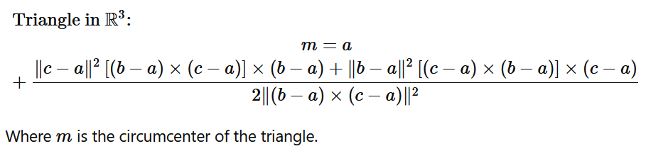
Spherical Voronoi regions are formed from Delaunay convex hull by connecting all the triangle circumcenters for the triangles touching one of the seeds.
Spherical Voronoi regions are formed from Delaunay convex hull by connecting all the triangle circumcenters for the triangles touching one of the seeds.
In[]:=
Clear[sqn,circCentTrig];sqn=Compile[{{arr,_Real,1}},Total[]];(*Normalizesbacktosphere*)circCentTrig=Compile[{{p1,_Real,1},{p2,_Real,1},{p3,_Real,1}},Block[{d2=p2-p1,d3=p3-p1,c},c=Cross[d2,d3];Normalize[p1+(sqn@d3*Cross[c,d2]+sqn@d2*Cross[-c,d3])/(2sqn@c)]]];
2
arr
Collecting triangles
Collecting triangles
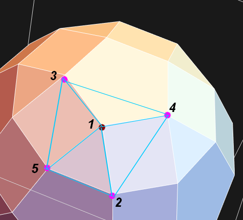
We should bear in mind that not only triangles, but also faces of any other form may connect at given vertex. So for vertex 1 Delaunay triangles are {1,3,4}, {1,4,2}, {1,2,5}, {1,5,3}.And they must be ordered, in a certain (but any) direction.To collect triangles, we need a special algorithm, for example.Here’s his open version, it works a bit slower.We can also use DualPolyhedron but it’s much slower.In this way, I tried to strike a balance between built-in functions, direct coding (to understand the subject) and performance.
In[]:=
(*Helpertocreatetablesofcell'slinks*)Clear[meshCellsLinks];meshCellsLinks[seeds_]:=Block[{chm=ConvexHullMesh@seeds,mc},ParallelTable[mc=First/@MeshCells[chm,c];Table[Select[mc,MemberQ[#,i]&],{i,Length@seeds}],{c,{1,2}}]];Clear[trigs];trigs[mc1_,mc2_]:=Block[{verts=DeleteDuplicates@Flatten@mc1,ngbs,res={},next},ngbs=Select[#,MemberQ[verts,#]&]&/@mc2;next=First@ngbs;Reap[Do[Sow@next;ngbs=DeleteCases[ngbs,next];next=SelectFirst[ngbs,Length@Intersection[#,next]==2&],{Length@ngbs}]][[2,1]]];
Make diagram
Make diagram
Output:
{
Coordinates of voronoi vertices,
List of matches {#seed, {##vertices}},
List of edges as sorted unique pairs,
If needRegions == True, list of spherical Voronoi regions or { }
}
Unfortunately, I couldn’t do without AppendTo here in a reasonable way.
Because calculating regions is a costly operation, it is done on demand.
{
Coordinates of voronoi vertices,
List of matches {#seed, {##vertices}},
List of edges as sorted unique pairs,
If needRegions == True, list of spherical Voronoi regions or { }
}
Unfortunately, I couldn’t do without AppendTo here in a reasonable way.
Because calculating regions is a costly operation, it is done on demand.
In[]:=
Clear[sphereVoronoiDiagram];sphereVoronoiDiagram[seeds_?MatrixQ,needRegions_:False]:=Block[{verts={},allTrigs={},vertsSeedsList={},edgesList={},regions={},p,thisSeedVerts,thisSeedEdges},(*NOParallel!!*)MapThread[(thisSeedVerts={};thisSeedEdges={};Table[p=FirstPosition[allTrigs,t,0];If[p=!=0,AppendTo[thisSeedVerts,First@p],AppendTo[allTrigs,t];AppendTo[thisSeedVerts,Length@allTrigs];AppendTo[verts,circCentTrig@@seeds[[t]]]],{t,Sort/@trigs[#1,#2]}];thisSeedEdges=Sort/@Partition[thisSeedVerts,2,1,1];edgesList=DeleteDuplicates@Join[edgesList,thisSeedEdges];AppendTo[vertsSeedsList,thisSeedVerts])&,meshCellsLinks@seeds];If[needRegions,regions=Table[ImplicitRegion[{And@@(#.{x,y,z}<=0&/@(#-seeds[[i]]&/@Delete[seeds,i])),x^2+y^2+z^2==1},{x,y,z}],{i,Length@seeds}]];{verts,vertsSeedsList,edgesList,regions}];
Graphics
Graphics
Exact parametric geodesic
Exact parametric geodesic
Approximated for graphics
In[]:=
Clear[geo,curves];geo[{p1_?VectorQ,p2_?VectorQ}]:=With[{w=ArcCos[p1.p2],u=Normalize[p2-p1(p1.p2)]},p1Cos[w#]+uSin[w#]&];curves[pts_,pairs_,nDiv_:20]:=Line@Table[Normalize@geo[pts[[#]]]@t,{t,Subdivide[0,1,nDiv]}]&/@pairs;
In[]:=
numSeeds=20;seeds=RandomPoint[Sphere[],numSeeds];svd=sphereVoronoiDiagram[seeds,True];
Construct a region for the selected seed:
Or make plain-style full diagram (with centroids):
Lloyd relaxation algorythm for spherical CVT
Lloyd relaxation algorythm for spherical CVT
The algorithm have to be fast, so we use a compiled function to calculate the centroid.
Centroid of spherical polygon
Centroid of spherical polygon
The polygon divide into triangles. The formula of a spherical triangle centroid is known.
Polygon has to be convex, vertices normalized and ordered.
Polygon has to be convex, vertices normalized and ordered.
One step
One step
Just short compact version of sphereVoronoiDiagram
Full Lloyd relaxation process
Full Lloyd relaxation process
This is the full process of Lloyd’s relaxation.
The sphereCVTProc function is running until a specified accuracy is achieved.
sphereCVTProcNum - given number of iterations.
Monitor shows the algorithm’s convergence, it can certainly be removed.
The sphereCVTProc function is running until a specified accuracy is achieved.
sphereCVTProcNum - given number of iterations.
Monitor shows the algorithm’s convergence, it can certainly be removed.
Are there different spherical CVT for given number of seeds?
Are there different spherical CVT for given number of seeds?
So second configuration is pure Icosahedron but first is not any standard polyhedron.
Voronoi energy
Voronoi energy
Voronoi tessellation energy function is the criterion for global CVT optimum.
For a small number of seeds, integration takes enough but acceptable time (5-6 sec).
For a small number of seeds, integration takes enough but acceptable time (5-6 sec).
As expected, configuration isomorphic of the icosahedron is a global energy minimizer (but it not strictly proven!)
Some conclusions
Some conclusions
A brief search showed that at N = 17 there are already three different non-isomorphic configurations with different total energies:
It is also interesting to look at the graphs formed by the vertices of the diagrams:
So we see that SphereCVT has the same questions as RectangleCVT:
- How many possible non-isormorphic stable CVTs for given N?
- In which cases are they isomorphic to such known configurations as solutions of Thomson and Tammes problems and other "spherical codes"?
- What about unstable (but centroidal) configurations?
- How many possible non-isormorphic stable CVTs for given N?
- In which cases are they isomorphic to such known configurations as solutions of Thomson and Tammes problems and other "spherical codes"?
- What about unstable (but centroidal) configurations?
CITE THIS NOTEBOOK
CITE THIS NOTEBOOK
Centroidal Voronoi diagrams on sphere
by Denis Ivanov
Wolfram Community, STAFF PICKS, July 28, 2026
https://community.wolfram.com/groups/-/m/t/3769381
by Denis Ivanov
Wolfram Community, STAFF PICKS, July 28, 2026
https://community.wolfram.com/groups/-/m/t/3769381