Solving the Maxwell-Stefan equations using two different methods
Authors: Housam Binous and Ahmed Bellagi
Authors: Housam Binous and Ahmed Bellagi
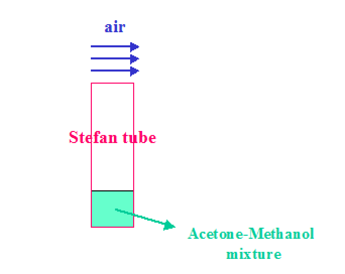
This problem is solved using Mathcad in Example 1.15 of Principles and Modern Applications of Mass Transfer Operations by Jaime Benitez, Wiley - Interscience, 2002.
Here, we computes the concentration profiles of components 1, 2 and 3 in the tube using the orthogonal collocation method (see Rice and Do, Applied Mathematics and Modeling for Chemical Engineers, Wiley, 1995) and the shooting method (developed by Brian Higgins, Chemical Engineering Department, University of California, Davis).
Both methods are found to give the same results as the digitized data from Carty and Schrodt, 1975.
References:
1 - Jaime Benitez, Principles and Modern Applications of Mass Transfer Operations, Wiley - Interscience, 2002.
2 - Rice and Do, Applied Mathematics and Modeling for Chemical Engineers, Wiley, 1995
3 - Carty and Schrodt, Concentration Profiles in Ternary Gaseous Diffusion, Ind. Eng. Chem. Fundamen., 1975, 14(3) , pp. 276–278.
4 - Binous and Bellagi, Orthogonal collocation methods using Mathematica© in the graduate chemical engineering curriculum, Comput Appl Eng Educ, 2016, 24, pp. 101-113.
In the bottom of a Stefan tube there is a quiescent liquid with a mixture of acetone (component 1) and methanol (component 2). Vapor that evaporates from this pool of liquid diffuses to the top of the tube. Air (component 3) keeps the mole fractions of components 1 and 2 equal to zero. =where c= , T=328.5 K , P=99.4 kPa , δ=0.24 m.The Maxwell-Stefan diffusion coefficients of the binary pairs are : = 8.48 /s, = 13.72 /s and = 19.91 /s.
F
ij
c
D
ij
δ
P
RT
D
12
2
mm
D
13
2
mm
D
23
2
mm
In[]:=
c=99.4/(328.5 8.314) 10^3
Out[]=
36.3949
In[]:=
δ=0.24
Out[]=
0.24
In[]:=
D
12
Out[]=
8.48
In[]:=
F
12
D
12
Out[]=
0.00128595
In[]:=
D
13
Out[]=
13.72
In[]:=
F
13
D
13
Out[]=
0.00208058
In[]:=
D
23
Out[]=
19.91
In[]:=
F
23
D
23
Out[]=
0.00301926
In[]:=
F
12
F
13
F
23
Since air does not dissolve in the liquid, we have N3=0
In[]:=
N3=0;
At x=δ (top of the Stefan tube) , Air (component 3) keeps the mole fractions of components 1 and 2 equal to zero.
At x=0 (the vapor liquid interface), the mole fractions of components 1 and 2 are equal to their equilibrium values at T=328.5 K and P=99.4 kPa (Carty and Schrodt, 1975).
At x=0 (the vapor liquid interface), the mole fractions of components 1 and 2 are equal to their equilibrium values at T=328.5 K and P=99.4 kPa (Carty and Schrodt, 1975).
In[]:=
Y[1,1]=0.319;Y[2,1]=0.528;Y[1,10]=0;Y[2,10]=0;
Orthogonal Collocation Method
Three internal collocation points (N=8)
In[]:=
solnodes=Solve[JacobiP[8,0,0,-1+2 u]==0.,u]
Out[]=
{{u0.0198551},{u0.101667},{u0.237234},{u0.408283},{u0.591717},{u0.762766},{u0.898333},{u0.980145}}
In[]:=
x[1]=1.010^-20;Table[x[i+1]=u/.solnodes[[i]],{i,1,8}];x[10]=1.;
Matrix Q and
-1
Q
In[]:=
Q=Chop[Table[Table[x[j]^(i-1),{i,1,10}],{j,1,10}]]
Out[]=
{{1.,0,0,0,0,0,0,0,0,0},{1.,0.0198551,0.000394224,7.82734×,1.55412×,3.08573×,0,0,0,0},{1.,0.101667,0.0103361,0.00105084,0.000106836,0.0000108616,1.10427×,1.12267×,1.14138×,1.16041×},{1.,0.237234,0.0562799,0.0133515,0.00316742,0.00075142,0.000178262,0.0000422898,0.0000100326,2.38007×},{1.,0.408283,0.166695,0.0680586,0.0277871,0.011345,0.00463197,0.00189115,0.000772125,0.000315245},{1.,0.591717,0.350129,0.207178,0.122591,0.072539,0.0429226,0.025398,0.0150285,0.0088926},{1.,0.762766,0.581812,0.443787,0.338506,0.258201,0.196947,0.150224,0.114586,0.0874023},{1.,0.898333,0.807003,0.724957,0.651253,0.585042,0.525563,0.472131,0.424131,0.381011},{1.,0.980145,0.960684,0.94161,0.922914,0.904589,0.886629,0.869025,0.85177,0.834858},{1.,1.,1.,1.,1.,1.,1.,1.,1.,1.}}
-6
10
-7
10
-9
10
-6
10
-7
10
-8
10
-9
10
-6
10
In[]:=
IQ=Inverse[Q]
Out[]=
{{1.,0.,0.,0.,0.,0.,0.,0.,0.,0.},{-72.9992,81.2227,-10.8522,3.92394,-2.12156,1.46378,-1.22021,1.22784,-1.6448,0.99965},{1331.98,-1838.48,685.496,-269.934,149.7,-104.402,87.4945,-88.2859,118.421,-71.9921},{-10499.9,15593.7,-7713.2,4089.45,-2459.76,1773.77,-1511.04,1537.67,-2070.7,1259.93},{43889.4,-67461.,38086.2,-23968.4,16256.,-12375.9,10834.8,-11184.5,15163.2,-9239.71},{-106720.,167194.,-101709.,71211.,-53318.2,43346.7,-39366.,41456.5,-56743.5,34649.3},{156154.,-247530.,157809.,-118654.,95871.5,-83002.8,78652.5,-84931.3,117702.,-72070.9},{-135562.,216570.,-142505.,112674.,-96545.7,88364.4,-87485.8,97253.6,-136846.,84083.1},{64349.,-103364.,69557.9,-57068.3,51198.8,-49153.5,50771.5,-58245.3,83433.6,-51479.6},{-12869.8,20755.2,-14200.3,11982.2,-11150.3,11150.3,-11982.2,14200.4,-20755.4,12869.9}}
Matrix C
In[]:=
Ci=Chop[Table[Table[(i-1)x[j]^(i-2),{i,1,10}],{j,1,10}]]
Out[]=
{{0,1.,0,0,0,0,0,0,0,0},{0,1.,0.0397101,0.00118267,0.0000313094,7.77062×,1.85144×,4.28871×,0,0},{0,1.,0.203334,0.0310084,0.00420336,0.000534178,0.0000651698,7.72987×,8.98138×,1.02725×},{0,1.,0.474468,0.16884,0.053406,0.0158371,0.00450852,0.00124784,0.000338319,0.0000902932},{0,1.,0.816565,0.500084,0.272234,0.138936,0.06807,0.0324238,0.0151292,0.00694913},{0,1.,1.18343,1.05039,0.82871,0.612953,0.435234,0.300458,0.203184,0.135256},{0,1.,1.52553,1.74544,1.77515,1.69253,1.5492,1.37863,1.20179,1.03127},{0,1.,1.79667,2.42101,2.89983,3.25627,3.51025,3.67894,3.77705,3.81718},{0,1.,1.96029,2.88205,3.76644,4.61457,5.42754,6.2064,6.9522,7.66593},{0,1.,2.,3.,4.,5.,6.,7.,8.,9.}}
-7
10
-8
10
-10
10
-6
10
-7
10
-7
10
Matrix A
In[]:=
A=Ci.IQ
Out[]=
{{-72.9992,81.2227,-10.8522,3.92394,-2.12156,1.46378,-1.22021,1.22784,-1.6448,0.99965},{-31.2298,24.672,8.36309,-2.65594,1.38322,-0.939552,0.777204,-0.778948,1.04153,-0.632742},{8.9143,-17.8652,4.36127,6.22432,-2.56099,1.60239,-1.27644,1.25532,-1.66392,1.00895},{-4.52745,7.96837,-8.74188,1.45206,5.44041,-2.62518,1.90287,-1.79269,2.33167,-1.40817},{2.82697,-4.79212,4.15351,-6.28245,0.379616,5.45156,-3.03151,2.59883,-3.25505,1.95065},{-1.9506,3.25496,-2.59877,3.03146,-5.45151,-0.37966,6.2825,-4.15357,4.79221,-2.82703},{1.40812,-2.33158,1.79263,-1.90282,2.62513,-5.44036,-1.45213,8.74197,-7.9685,4.52753},{-1.00886,1.66377,-1.25521,1.27634,-1.60229,2.56088,-6.22419,-4.36145,17.8655,-8.91447},{0.632626,-1.04134,0.778814,-0.777081,0.939424,-1.38307,2.65576,-8.36285,-24.6724,31.2301},{-0.999985,1.64535,-1.22824,1.22058,-1.46418,2.12202,-3.92451,10.8529,-81.2239,73.}}
In[]:=
Ci.IQ//MatrixForm
Out[]//MatrixForm=
-72.9992 | 81.2227 | -10.8522 | 3.92394 | -2.12156 | 1.46378 | -1.22021 | 1.22784 | -1.6448 | 0.99965 |
-31.2298 | 24.672 | 8.36309 | -2.65594 | 1.38322 | -0.939552 | 0.777204 | -0.778948 | 1.04153 | -0.632742 |
8.9143 | -17.8652 | 4.36127 | 6.22432 | -2.56099 | 1.60239 | -1.27644 | 1.25532 | -1.66392 | 1.00895 |
-4.52745 | 7.96837 | -8.74188 | 1.45206 | 5.44041 | -2.62518 | 1.90287 | -1.79269 | 2.33167 | -1.40817 |
2.82697 | -4.79212 | 4.15351 | -6.28245 | 0.379616 | 5.45156 | -3.03151 | 2.59883 | -3.25505 | 1.95065 |
-1.9506 | 3.25496 | -2.59877 | 3.03146 | -5.45151 | -0.37966 | 6.2825 | -4.15357 | 4.79221 | -2.82703 |
1.40812 | -2.33158 | 1.79263 | -1.90282 | 2.62513 | -5.44036 | -1.45213 | 8.74197 | -7.9685 | 4.52753 |
-1.00886 | 1.66377 | -1.25521 | 1.27634 | -1.60229 | 2.56088 | -6.22419 | -4.36145 | 17.8655 | -8.91447 |
0.632626 | -1.04134 | 0.778814 | -0.777081 | 0.939424 | -1.38307 | 2.65576 | -8.36285 | -24.6724 | 31.2301 |
-0.999985 | 1.64535 | -1.22824 | 1.22058 | -1.46418 | 2.12202 | -3.92451 | 10.8529 | -81.2239 | 73. |
Matrix D
In[]:=
Di=Chop[Table[Table[(i-1)(i-2)x[j]^(i-3),{i,1,10}],{j,1,10}]]
Out[]=
{{0,0,2.,0,0,0,0,0,0,0},{0,0,2.,0.11913,0.00473069,0.000156547,4.66237×,1.296×,3.43097×,0},{0,0,2.,0.610001,0.124034,0.0210168,0.00320507,0.000456188,0.0000618389,8.08324×},{0,0,2.,1.4234,0.675358,0.26703,0.0950227,0.0315596,0.00998268,0.00304487},{0,0,2.,2.4497,2.00034,1.36117,0.833614,0.47649,0.25939,0.136163},{0,0,2.,3.5503,4.20155,4.14355,3.67772,3.04664,2.40366,1.82866},{0,0,2.,4.5766,6.98175,8.87573,10.1552,10.8444,11.029,10.8161},{0,0,2.,5.39,9.68403,14.4991,19.5376,24.5718,29.4315,33.9934},{0,0,2.,5.88087,11.5282,18.8322,27.6874,37.9928,49.6512,62.5698},{0,0,2.,6.,12.,20.,30.,42.,56.,72.}}
-6
10
-7
10
-9
10
-6
10
Matrix B
In[]:=
B=Di.IQ
Out[]=
{{2663.97,-3676.96,1370.99,-539.868,299.4,-208.804,174.989,-176.572,236.842,-143.984},{1604.74,-2113.36,617.084,-155.468,75.3567,-49.6309,40.4272,-40.1932,53.5392,-32.499},{-97.6039,280.904,-302.741,146.116,-39.041,20.5147,-14.9934,14.099,-18.299,11.0452},{25.0198,-50.1712,103.58,-142.81,79.4117,-22.4348,12.7676,-10.6293,13.0481,-7.78154},{-11.7016,21.0359,-23.9389,68.6879,-105.054,63.5776,-19.4053,12.5794,-13.8552,8.0741},{8.07406,-13.8552,12.5794,-19.4053,63.5776,-105.054,68.688,-23.939,21.0361,-11.7017},{-7.78163,13.0483,-10.6294,12.7677,-22.435,79.4119,-142.81,103.58,-50.1719,25.0202},{11.0462,-18.3007,14.1003,-14.9946,20.5159,-39.0425,146.117,-302.743,280.908,-97.6065},{-32.5077,53.5533,-40.2034,40.4368,-49.6411,75.3686,-155.482,617.104,-2113.39,1604.76},{-143.998,236.864,-176.588,175.005,-208.821,299.42,-539.893,1371.03,-3677.01,2664.}}
In[]:=
Di.IQ//MatrixForm
Out[]//MatrixForm=
2663.97 | -3676.96 | 1370.99 | -539.868 | 299.4 | -208.804 | 174.989 | -176.572 | 236.842 | -143.984 |
1604.74 | -2113.36 | 617.084 | -155.468 | 75.3567 | -49.6309 | 40.4272 | -40.1932 | 53.5392 | -32.499 |
-97.6039 | 280.904 | -302.741 | 146.116 | -39.041 | 20.5147 | -14.9934 | 14.099 | -18.299 | 11.0452 |
25.0198 | -50.1712 | 103.58 | -142.81 | 79.4117 | -22.4348 | 12.7676 | -10.6293 | 13.0481 | -7.78154 |
-11.7016 | 21.0359 | -23.9389 | 68.6879 | -105.054 | 63.5776 | -19.4053 | 12.5794 | -13.8552 | 8.0741 |
8.07406 | -13.8552 | 12.5794 | -19.4053 | 63.5776 | -105.054 | 68.688 | -23.939 | 21.0361 | -11.7017 |
-7.78163 | 13.0483 | -10.6294 | 12.7677 | -22.435 | 79.4119 | -142.81 | 103.58 | -50.1719 | 25.0202 |
11.0462 | -18.3007 | 14.1003 | -14.9946 | 20.5159 | -39.0425 | 146.117 | -302.743 | 280.908 | -97.6065 |
-32.5077 | 53.5533 | -40.2034 | 40.4368 | -49.6411 | 75.3686 | -155.482 | 617.104 | -2113.39 | 1604.76 |
-143.998 | 236.864 | -176.588 | 175.005 | -208.821 | 299.42 | -539.893 | 1371.03 | -3677.01 | 2664. |
Maxwell-Stefan relations written using the orthogonal collocation method gives a set of simultaneous algebraic equations that are easily solved using FindRoot.
In[]:=
Fori=1,i<11,eq[1,i]=A[[i,j]]Y[1,j]1(Y[1,i]N2-Y[2,i]N1)+1(Y[1,i]N3-(1-Y[1,i]-Y[2,i])N1);i++
10
∑
j=1
F
12
F
13
In[]:=
Fori=1,i<11,eq[2,i]=A[[i,j]]Y[2,j]1(Y[2,i]N1-Y[1,i]N2)+1(Y[2,i]N3-(1-Y[1,i]-Y[2,i])N2);i++
10
∑
j=1
F
12
F
23
In[]:=
UNKNOWNS=Join[Table[{Y[1,i],0.2},{i,2,9}],Table[{Y[2,i],0.4},{i,2,9}],{{N1,1.28610^-3},{N2,1.28610^-3}}]
Out[]=
{{Y[1,2],0.2},{Y[1,3],0.2},{Y[1,4],0.2},{Y[1,5],0.2},{Y[1,6],0.2},{Y[1,7],0.2},{Y[1,8],0.2},{Y[1,9],0.2},{Y[2,2],0.4},{Y[2,3],0.4},{Y[2,4],0.4},{Y[2,5],0.4},{Y[2,6],0.4},{Y[2,7],0.4},{Y[2,8],0.4},{Y[2,9],0.4},{N1,0.001286},{N2,0.001286}}
In[]:=
SYS=Flatten[Join[Table[eq[1,i],{i,2,10}],Table[eq[2,i],{i,2,10}]]];
In[]:=
sol=FindRoot[SYS,UNKNOWNS]
Out[]=
{Y[1,2]0.317246,Y[1,3]0.309214,Y[1,4]0.292487,Y[1,5]0.263148,Y[1,6]0.216525,Y[1,7]0.151042,Y[1,8]0.0759242,Y[1,9]0.0164407,Y[2,2]0.523943,Y[2,3]0.505611,Y[2,4]0.468672,Y[2,5]0.40757,Y[2,6]0.318827,Y[2,7]0.208367,Y[2,8]0.0978282,Y[2,9]0.0201474,N10.00176837,N20.00310217}
Plotting the results
In[]:=
Tbl1=Table[{δ x[i],Y[1,i]}/.sol,{i,1,10}]
In[]:=
Tbl2=Table[{δ x[i],Y[2,i]}/.sol,{i,1,10}]
In[]:=
Tbl3=Table[{δ x[i],1-Y[1,i]-Y[2,i]}/.sol,{i,1,10}]
In[]:=
plt1=ListPlot[Tbl1,PlotStyle->RGBColor[1,0,0],Joined->True,PlotLabel->Row[{Style["Air",Green,14],Style["Acetone",Red,14],Style["Methanol",Blue,14]},"---"]];
In[]:=
plt2=ListPlot[Tbl2,PlotStyle->RGBColor[0,0,1],Joined->True];
In[]:=
plt3=ListPlot[Tbl3,PlotStyle->RGBColor[0,1,0],Joined->True];
In[]:=
Show[plt1,plt2,plt3,Frame->True,GridLines-> Automatic,ImageSize->450{1,1},AspectRatio->1,PlotRange->All,FrameLabel->{Style["position",16],Style["mole fraction",16]}]
In[]:=
plt4=ListPlot[Tbl1,PlotStyle->{PointSize[0.02],RGBColor[1,0,0]},PlotLabel->Row[{Style["Air",Green,14],Style["Acetone",Red,14],Style["Methanol",Blue,14]},"---"]];
In[]:=
plt5=ListPlot[Tbl2,PlotStyle->{PointSize[0.02],RGBColor[0,0,1]}];
In[]:=
plt6=ListPlot[Tbl3,PlotStyle->{PointSize[0.02],RGBColor[0,1,0]}];
In[]:=
Show[plt4,plt5,plt6,Frame->True,GridLines-> Automatic,ImageSize->450{1,1},AspectRatio->1,PlotRange->All,FrameLabel->{Style["position",16],Style["mole fraction",16]}]
Shooting Method
Acknowledgement :
Since in this problem we have split boundary conditions, its resolution is based on the Shooting Method developed in Mathematica by Professor Brian Higgins (Chemical Engineering Department, University of California, Davis ).
Acknowledgement :
Since in this problem we have split boundary conditions, its resolution is based on the Shooting Method developed in Mathematica by Professor Brian Higgins (Chemical Engineering Department, University of California, Davis ).
Solving the Maxwell-Stefan equations using the shooting method
In[]:=
myODEsoln[N1_,N2_]:=NDSolve[system[N1,N2],{Y1[x],Y2[x]},{x,0,1}]
In[]:=
yend1[N1_?NumericQ,N2_?NumericQ]:=Flatten[(Y1[x]/.myODEsoln[N1,N2])/.x1]
yend2[N1_?NumericQ,N2_?NumericQ]:=Flatten[(Y2[x]/.myODEsoln[N1,N2])/.x1]
yend2[N1_?NumericQ,N2_?NumericQ]:=Flatten[(Y2[x]/.myODEsoln[N1,N2])/.x1]
In[]:=
bc=FindRoot[{yend1[N1,N2]0,yend2[N1,N2]0},{N1,0.0015},{N2,0.007}];
c={N1,N2}/.bc;
bc=FindRoot[{yend1[N1,N2]0,yend2[N1,N2]0},{N1,0.0015},{N2,0.007}];
c={N1,N2}/.bc;
In[]:=
c
In[]:=
c[[1]]
In[]:=
c[[2]]
Plotting the results
In[]:=
plt7=Plot[Evaluate[Y1[x]/.myODEsoln[c[[1]],c[[2]]]/.x->u/δ],{u,0,δ},PlotStyle->RGBColor[1,0,0]
,PlotLabel->Row[{Style["Air",Green,14],Style["Acetone",Red,14],Style["Methanol",Blue,14]},"---"]];
,PlotLabel->Row[{Style["Air",Green,14],Style["Acetone",Red,14],Style["Methanol",Blue,14]},"---"]];
In[]:=
plt8=Plot[Evaluate[Y2[x]/.myODEsoln[c[[1]],c[[2]]]/.x->u/δ],{u,0,δ},PlotStyle->RGBColor[0,0,1]];
In[]:=
plt9=Plot[Evaluate[(1-Y1[x]-Y2[x])/.myODEsoln[c[[1]],c[[2]]]/.x->u/δ],{u,0,δ},PlotStyle->RGBColor[0,1,0]];
In[]:=
Show[plt7,plt8,plt9,Frame->True,GridLines-> Automatic,ImageSize->450{1,1},AspectRatio->1,PlotRange->All,FrameLabel->{Style["position",16],Style["mole fraction",16]}]
In[]:=
Show[plt4,plt5,plt6,plt7,plt8,plt9,Frame->True,GridLines-> Automatic,ImageSize->450{1,1},AspectRatio->1,
PlotRange->All,FrameLabel->{Style["position",16],Style["mole fraction",16]}]
PlotRange->All,FrameLabel->{Style["position",16],Style["mole fraction",16]}]
Acknowledgements: Example 1.15 of Principles and Modern Applications of Mass Transfer Operations by Jaime Benitez, Wiley-Interscience, 2002.