Finding zeros with domain coloring and winding numbers
by Garrett Dubofsky
Western Washington University
by Garrett Dubofsky
Western Washington University
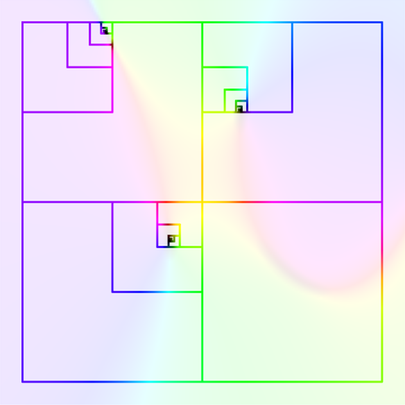
Given a 2-dimensional transformation, we shall start by plotting its domain coloring. Specifically, every point on the plane takes the hue of where that point’s transformation lands on a color wheel centered at the origin. The winding number of any boundary on this domain is representative of how many loops of the color spectrum are completed when moving clockwise along the boundary. If the winding number is a nonzero integer, the boundary can be repeatedly halved as it converges onto a zero of the transformation. We seek to create this process visually and mathematically using the Wolfram Language.
Domain Coloring
Domain Coloring
In many areas of math, it is important to determine the points at which an equation outputs a zero. These zeros can represent extrema, intersections, optimal values, and much more. There are many methods available to locate the zeros of simplistic equations but it becomes more difficult as the equations increase in complexity. In this project, we seek to discover a method for finding zeros of a particular type of equation – a continuous 2-dimensional transformation – with a process involving domain coloring and winding numbers.
It is a challenge to visualize 2-dimensional transformations in our 3-dimensional world. This task might sound intuitive but these 2D transformations require two inputs and two outputs, resulting in a total of 4 components. We must overcome this obstacle if we wish to visualize our search for zeros. Let us define a 2D transformation to use as an example for our computations; the Q function is designed to be continuous and differentiable while remaining difficult to algebraically manipulate. Notice that the zeros of this type of transformation are points that map to the coordinates . For the sake of innovation, I did not determine the zeros of Q before starting this project.
{0,0}
In[]:=
Q[{x_,y_}]={+-5-2x*y+3+Cos[y],+y*(x-3)+2y-3-Sin[y]};
3
x
2
y
2
x
2
y
There exist a variety of potential ways to visualize the above transformation, some of which work better than others. A common representation of 2D transformations is a vector graph, which uses an arbitrary number of vectors located at different points to give the direction that Q sends each point. Each vector’s magnitude corresponds to the euclidean distance the given point travels.
Plot the vector graph of Q with vector scaling enabled.
Out[]=
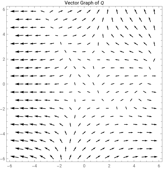
While this graph clearly explains the directions that Q induces, we cannot determine where each point travels. This is an insufficient amount of information for our goal of finding zeros. To compensate, we will introduce a new form of visualization: domain coloring. The process of domain coloring is unorthodox, a little unintuitive, but ultimately beautiful. Consider placing a hue wheel centered at the origin and covering the entire plane. Points closer to the origin shall be shaded darker to exaggerate their importance.
2
Use ColorFunction to apply the domain coloring to the plane.
Out[]=
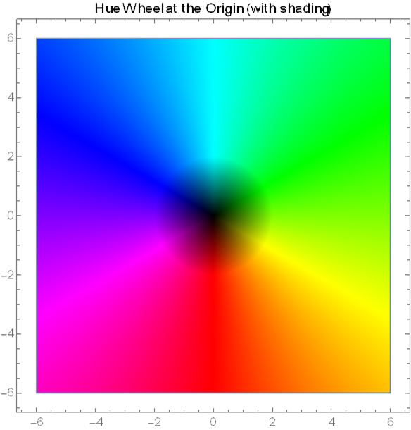
To find the domain coloring of the Q transformation, we color each point on the plane according to where its transformation lands on the hue wheel. In other words, the transformed point is “painted” by the hue wheel before returning to its starting location. Let us implement this process using a grid of points and the Q transformation:
Assigning each point on the discretized plane its Q-transformed hue.
Out[]=
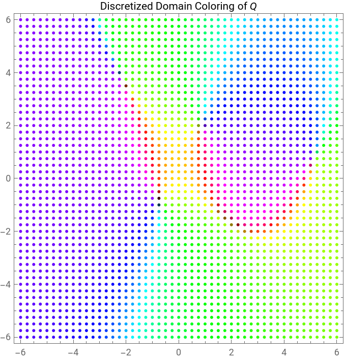
This process can be improved further by increasing the density of points. With enough detail, we successfully encode both a transformed point’s direction and distance from the origin.
Recreating the previous graphic with indistinguishable points.
Out[]=
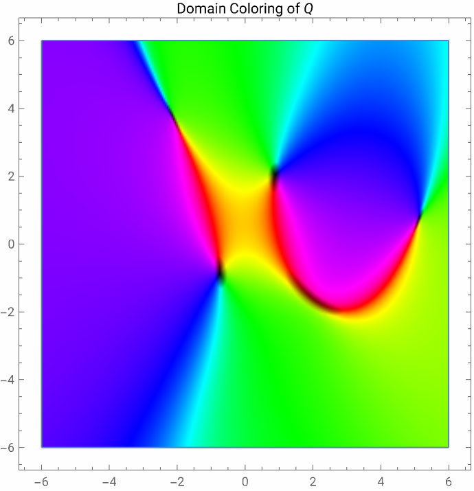
The above graphic is called the domain coloring of Q. The shading makes is clear which points the Q transformation sends close to the origin. While this approaches our goal of finding the zeros of Q, domain coloring not only required evaluating the transformation over an entire area of the plane but it does not produce numerical estimates. Next, we will uncover a method that overcomes these obstacles.
Determining the Winding Number
Determining the Winding Number
Instead of investigating an entire area, let us select just a closed boundary. This is a significant computational improvement; analyzing a perimeter instead of an area dramatically reduces the number of processed points. Any arbitrary shape will suffice but few will make later processes significantly easier to compute. Therefore, we will limit our analysis to rectangular boundaries. Such a rectangle can be projected atop the above graphic to isolate the domain coloring of Q along its perimeter.
Plotting the domain coloring of Q along a rectangle’s perimeter.
Out[]=
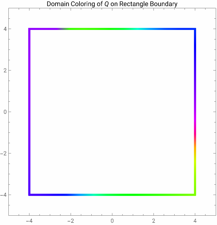
Before we can describe the meaning of a winding number, it is important to first describe what we are “winding”. Simply enough, we are winding around the hue wheel. This can be interpreted as the angular movement of an arrow that points towards its color on a surrounding hue wheel. Moving in the “ROYGBIV” direction will increase the winding number, whereas moving in the opposite direction will decrease it.
Not only do we have to establish the concept of winding, we need to calculate its numeric value. In the Wolfram Language, each hue is designed a unique value between 0 and 1. Therefore, we can plot the hue value along the boundary as we move clockwise starting in the top left corner. By coloring the curve accordingly, the correspondence between color and value becomes clear. Asymptotic discontinuities occur because the hue value of red is both 0 and 1. Thus, moving directly between 0 and 1 does not constitute as a discontinuity when moving around the hue wheel. In other words, the hue value may be discontinuous but the color order is not. Since we start and end at the same location, the number of complete hue wheel rotations (the winding number) must be an integer.
An animation showcasing all three processes combined.
Out[]=
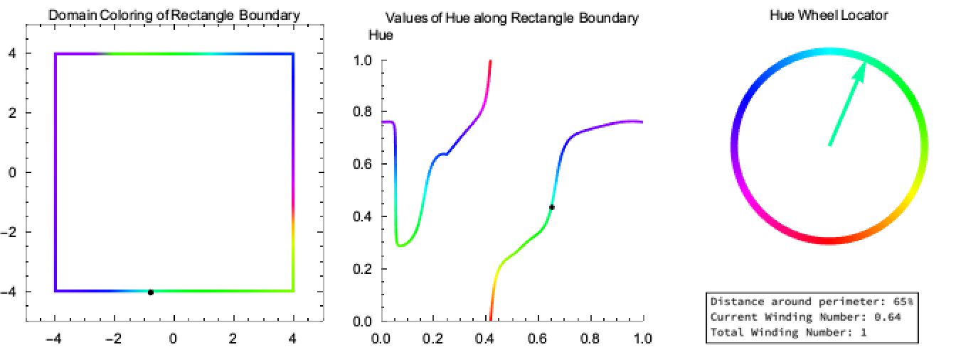

The winding number is equivalent to the net change of the hue value across the rectangle’s perimeter. Since the curve of hue values is typically discontinuous and non-differentiable, we rely on a discretization to find the winding number. That is, the horizontal axis partitioned into a large number of equal-length intervals and the change in the function across each interval. The summation of these differences produces the net change of the hue value across the boundary -- the winding number.
Decreasing the Boundary
Decreasing the Boundary
Properties of Winding Numbers
Properties of Winding Numbers
Now we can elaborate why the winding number is an important tool for finding zeros of 2D transformations. Notice that zeros are the only points with the property that if we zoom infinitely close to the point, we are guaranteed that the surrounding domain coloring shall pass through the entire hue spectrum. This property directly follows from the requirement that the 2D transformation is continuous, which we discovered also implies that the domain coloring is color-continuous (no jumps in hue between two points). Since the domain coloring of the plane places the origin in the center of the hue wheel, any point that maps to the origin must also retain this quality.
Additionally, halving a boundary with a nonzero winding number is guaranteed to produce at least one smaller boundary with a nonzero winding number. This is a result from the fact that winding numbers are integers along with the addition properties discussed later. Since a nonzero winding number implies that the boundary passes through the entire hue spectrum, we can repeatedly apply this process until we obtain an infinitesimally small boundary that still passes through all colors. As we stated earlier, this infinitely small boundary (which can be thought of as a point) must be a zero. Therefore, any closed boundary with a nonzero winding number must contain a zero. We specify a nonzero winding number because it is possible to create a boundary that passes through the entire spectrum but, when split in two, neither of its halves does the same. On the other hand, a boundary with a zero winding number may actually contain a zero. This scenario is captured with a large boundary around the domain coloring of the Q below:
Determining the winding number of the 11x11 square centered at the origin.
Although this large boundary has a winding number of zero, we will discover shortly that the region it encompasses surrounds at least one zero. This phenomenon is created by two regions with nonzero winding numbers, one positive and one negative, cancelling the other’s value. The process of winding number addition can be depicted below, where it is important to remember that the hue value along a boundary is evaluated clockwise. The red and blue colors only identify the winding orientation and do not represent the domain coloring.
Animation of the winding number addition of two rectangular boundaries using a table of points.
Due to the common clockwise orientation, it is clear that the winding of the shared edge will cancel when the boundaries and combined. Therefore, the winding number of the large boundary is equivalent to the sum of the winding number of the two smaller boundaries.
Computing the winding numbers of the red, blue, and red-blue boundaries from above.
Zeroing In on Zeros
Zeroing In on Zeros
As discussed above, the first step of our analysis requires finding a boundary with a nonzero winding number. This boundary is then halved and it is determined which half still has the desired nonzero winding number. This process is repeated until we obtain the desired boundary area, which results in a small region that must contain a zero. At this stage, we can approximate the exact location of the zero by using the center of the rectangle. However, a rectangular boundary shape means that halving the boundary repeatedly using only one axis will result in a very elongated strip. This is undesirable because we will only be able to approximate one coordinate of the zero while the other remains unknown. Thus, our halving process will alternate between the axes.
Confirming this region satisfies our nonzero winding number requirement.
A list of rectangular boundary corners found by applying the halving process until the area fell below the cutoff value.
Therefore, we have an estimation of a zero at the following coordinates:
Finding the midpoint of the last region.
We can determine the accuracy of this estimation by evaluating the output of Q and its euclidean norm at this coordinate. Ideally, the norm value of the zero estimate is close to 0.
Plugging in the estimated zero point into the Q function, plus its norm.
This is very accurate! We can visually depict the utility of this process by plotting the rectangular search boundaries as they approach the zero:
Graphing the outputs of the search boundaries in one image.
Remember that darker hues correlate to points that Q sends near the origin. Thus, darker shading corresponds to smaller norm values. We can see above that the boundary area decreases quickly, but what about the estimation error? To investigate how quickly this error decreases, we can plot each estimation’s norm value against the number of iterations:
Plots of the norm value vs. number of iterations, one with log scaling.
Notice that the logarithmically scaled plot is linear, implying that the estimation’s error decreases exponentially!
Repeating the investigation with a new initial boundary.
It should be noted that multiple (potentially infinite) initial boundaries can converge to the same zero:
Determining the winding number and finding the zero estimate on a new boundary.
Concluding Remarks
Concluding Remarks
Future Endeavours
Future Endeavours
Let us show the respective domain coloring and find a boundary with a nonzero winding number:
Plotting the domain coloring of A and finding the winding number of the gray boundary.
Even though the boundary passes through two non-differentiable points, it is still possible to find a zero in this region:
Zero estimation for the boundary on A.
Other areas of exploration include finding winding numbers of non-rectangular boundaries. We chose to investigate rectangular boundaries for their convenience, but any closed curve has a winding number. Future endeavors would involve redefining findWR for a curve that is formed from any number of points. Additionally, the functions we defined only produce the coordinates of one boundary, even though both boundaries might have nonzero winding numbers. These functions also require that the initial boundary has a nonzero winding number. Addressing these two issues would improve the reliability of finding all zeros in a given region.
Potential Issues
Potential Issues
This methodology is not a perfect process. For instance, lots of evaluations are required for finding a winding number depending on the level of accuracy. The nature of winding number addition also leads to instances where an initial region has a winding number of zero but encloses multiple zeros of the transformation. Other processes that rely on Newton’s method have advantages and disadvantages over winding numbers; Newton’s method may compute faster but winding numbers do not require finding a derivative.
Winding number of a specific boundary on A.
Domain coloring of A around the specific boundary. The zero is highlighted in black.
Therefore, a boundary that passes through a zero does not produce a sensible winding number. Although the objective is to find zeros, one must be careful that the search boundaries surround the zero instead of intersecting it. For this reason, any boundary with a non-integer winding number should be thoroughly investigated.
Conclusion
Conclusion
Out of the many methods available to find zeros of 2D transformations, none are as visually stunning as domain coloring and winding numbers. By taking an unorthodox approach to zero estimation, we have revealed new ways to visualize 2D transformations, uncover complexities of relatively simplistic concepts, and estimate zeros with an exponentially-decaying error. This process brings more color to the world of math and highlights how the same result can be approached in a myriad of ways. Many more avenues of exploration remain for this intriguing and beautiful method, and it is very exciting to see what awaits.
Acknowledgments
Acknowledgments
In no particular order, I would like to acknowledge those who inspired, encouraged, and assisted me throughout the process of building this document:
◼
My mentor, Clayton Shonkwiler, give very useful feedback, suggested innovative visualizations, and provided crucial code assistance. His expertise in Mathematica visualizations was a huge inspiration and crucial for the many pitfalls I encountered.
◼
Although Paul Abbott started my journey in the Wolfram Summer School program, his involvement did not stop there. His dedication to my success drove me to achieve something beyond what I thought I could accomplish. His supply of tips, tools, and resources kept me both excited about my project and the world of math as a whole.
◼
I appreciate Erin Cherry’s patience, tenacity, and commitment to making the WSS run smoothly. She kept everyone on track and made sure to remind me of important deadlines. Many important events would have been missed without her guidance.
◼
It was a pleasure to meet Stephen Wolfram and hear his feedback on my project topic. Dr. Wolfram inspired me during my educational journey and it was amazing to participate in his program.
◼
Branko Ćurgus made me the mathematician I am today. He taught me many fundamental math concepts, one of which being the Wolfram Language. Without his guidance, I would not have had the opportunity to participate in the WSS.
◼
I would like to thank my girlfriend Samantha Kirlin and my parents for listening, assisting, and supporting me throughout the duration of this project.
References
References
◼
Grant Sanderson’s (3Blue1Brown) YouTube video: https://youtu.be/b7FxPsqfkOY
Code
Code
This code consists of function definitions and lists of frames used for the animations. They are listed in order of use throughout the document.