Wolfram Cloud Page

"Figure 1. The numerically optimised sofa (blue) sweeping through a unit-width L-corridor. The orange L is the corridor in the sofa-fixed frame as it rotates from θ = 0° (fully in the horizontal arm) to θ = 90° (fully in the vertical arm). Its area, 2.2197, matches Gerver's known optimum to four decimals. The rest of the notebook explains how the optimiser found this shape, sweeps the bend angle across (0, π), and tries a first numerical attack on the 3D analogue."

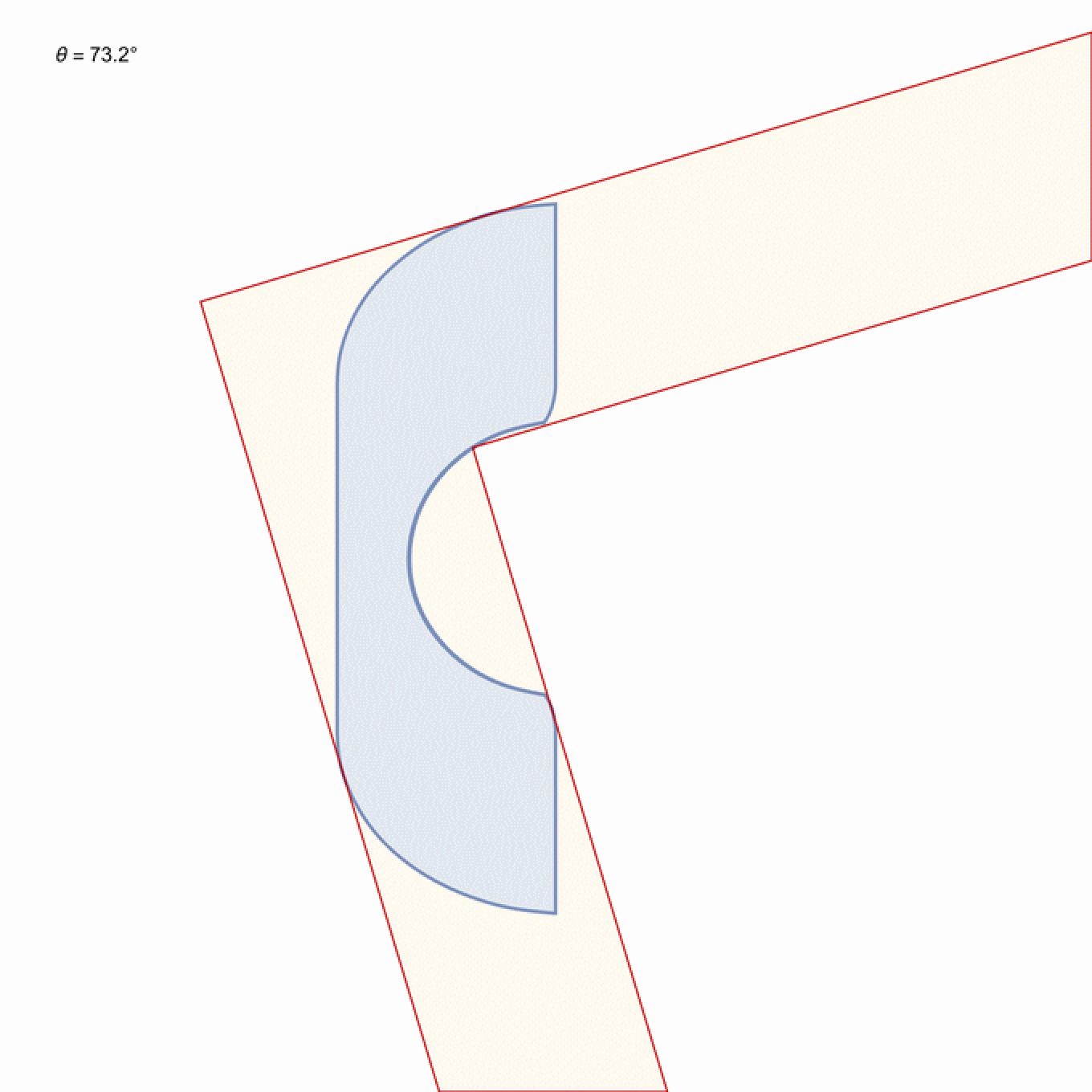
The moving sofa problem asks for the largest 2D rigid body that can slide through an L-shaped corridor of unit width while making a 90° turn. Hammersley (1968) constructed a sofa of area

π/2+2/π≈2.207

; Gerver (1992) refined this to an 18-arc shape of area

2.21953

, and Baek (2024) recently proved that Gerver's sofa is optimal. This notebook reproduces a Gerver-class shape from scratch with a small Python optimiser (cubic-spline trajectory of the inner corner of the L; Nelder–Mead on ≈20 parameters), gives a literal Wolfram-Language port of the same algorithm, sweeps the corridor bend angle across (0, π) and reports the resulting areas, and ends with a short discussion of what changes (and what is open) in three dimensions. https://github.com/mthiel74/SofaProblem

"Figure 2. The optimised sofa (light blue), area ≈ 2.2197, together with the inner-corner trajectory the optimiser discovered (dashed orange). Width 1, length 2 + 4/π ≈ 3.27. The sofa is essentially Gerver's shape."

1. The puzzle

An L-shaped corridor of unit width: the horizontal arm is the strip

{(x,y)}:x≥0,y∈[0,1]

and the vertical arm is its reflection across

y=x

. A connected planar body

is a sofa if there is a continuous rigid motion of

starting deep in the horizontal arm and ending deep in the vertical arm, with

contained in the corridor at every instant. What is the

suparea(S)

A trivial unit square gives area 1; a half-disk of radius 1 fits and gives area

π/2≈1.571

. Hammersley's 1968 construction — a rectangle with a semicircular notch cut from its bottom — gives

π/2+2/π≈2.207

. Gerver (1992) replaced the rectangle with an 18-arc shape and got

2.21953

; the recent proof by Baek (arXiv:2411.19826, 2024) shows that

2.21953...

is the exact answer.

2. The sofa-fixed-frame formulation

Instead of moving the sofa through a fixed corridor, fix the sofa and let the corridor rotate and translate around it. The motion is parameterised by an angle

∈ [0, π/2]; in the sofa-fixed frame the world's axes are rotated by

-θ

(θ)=(cosθ,-sinθ),

(θ)=(sinθ,cosθ)

Each pose places an L-shaped corridor

L(θ)

in the sofa frame. The largest sofa consistent with a given trajectory

C(θ)

of the inner corner is the polygon intersection

max

(C)=

⋂

θ∈[0,π/2]

L(θ;C(θ))

and we maximise its area over the trajectory

3. A Wolfram-Language exploration

Discretise the integral above: pick a dense set of

samples, build the L-corridor at each sample, intersect them all. The trajectory

C(θ)

is the parameter we optimise. As a first pass, fit a parametric trajectory by hand: a translation of the form

T(α)=amp·sign(cos2α)·|cos2α

,rotationϕ(α)=...

Set up the corridor as a region and look at one corridor pose:

reg=RegionUnion[DiscretizeGraphics[Graphics@Rectangle[{-5,-1},{2,1}]],DiscretizeGraphics[Graphics@Rectangle[{0,-1},{2,-6}]]];

Manipulate[RegionPlot[{reg,TransformedRegion[TransformedRegion[reg,TranslationTransform[{-2Cos[α]+1,-1+2Cos[α]}]],RotationTransform[-α+Pi/4,{0,-1}]]},PlotRange->{{-6,6},{-6,6}}],{α,0,Pi/2}]

Tune the two exponents and the amplitude by hand and integrate every pose:

(*hand-tunedparametrictrajectorytheuserconvergedon;amp≈1.22,exp1≈0.68,exp2≈0.53*)amp=1.22;exp1=0.68;exp2=0.53;regs=Table[TransformedRegion[TransformedRegion[reg,TranslationTransform[{-ampSign[Cos[2α]]Abs[Cos[2α]]^exp1,ampSign[Cos[2α]]Abs[Cos[2α]]^exp1}]],RotationTransform[Sign[-α+Pi/4.](Abs[-α+Pi/4.]4/Pi)^exp2Pi/4.,{0,-1}]],{α,0,Pi/2,0.015}];sofa=Fold[RegionIntersection,regs];Area[sofa]/4(*divideby4becauseregisona2-unit-widecorridor*)

Trial and error converges to area

≈2.14

on a 2-unit-wide corridor (so

≈2.14

on the unit-width problem after the divide-by-4). This is comfortably above the simple half-disk of radius 1 (area

π/2

) but still short of Hammersley’s 2.207 — showing how much is left on the table once we move away from low-dimensional hand-tuned curves.

4. A Python optimiser as a comparison baseline

Before writing the Wolfram-native optimiser, it's useful to have an independent implementation in another language to compare against. We use Python through Wolfram's ExternalLanguage interface: the cell below is a real ExternalLanguage Python cell, executed via ExternalEvaluate (requires RegisterExternalEvaluator["Python", ...] if you haven't done it once already). The Wolfram-native version follows in Section 5, and we'll see that the two reach the same Gerver-class optimum to four decimals — confirmation that the algorithm, not the language, is what's doing the work.

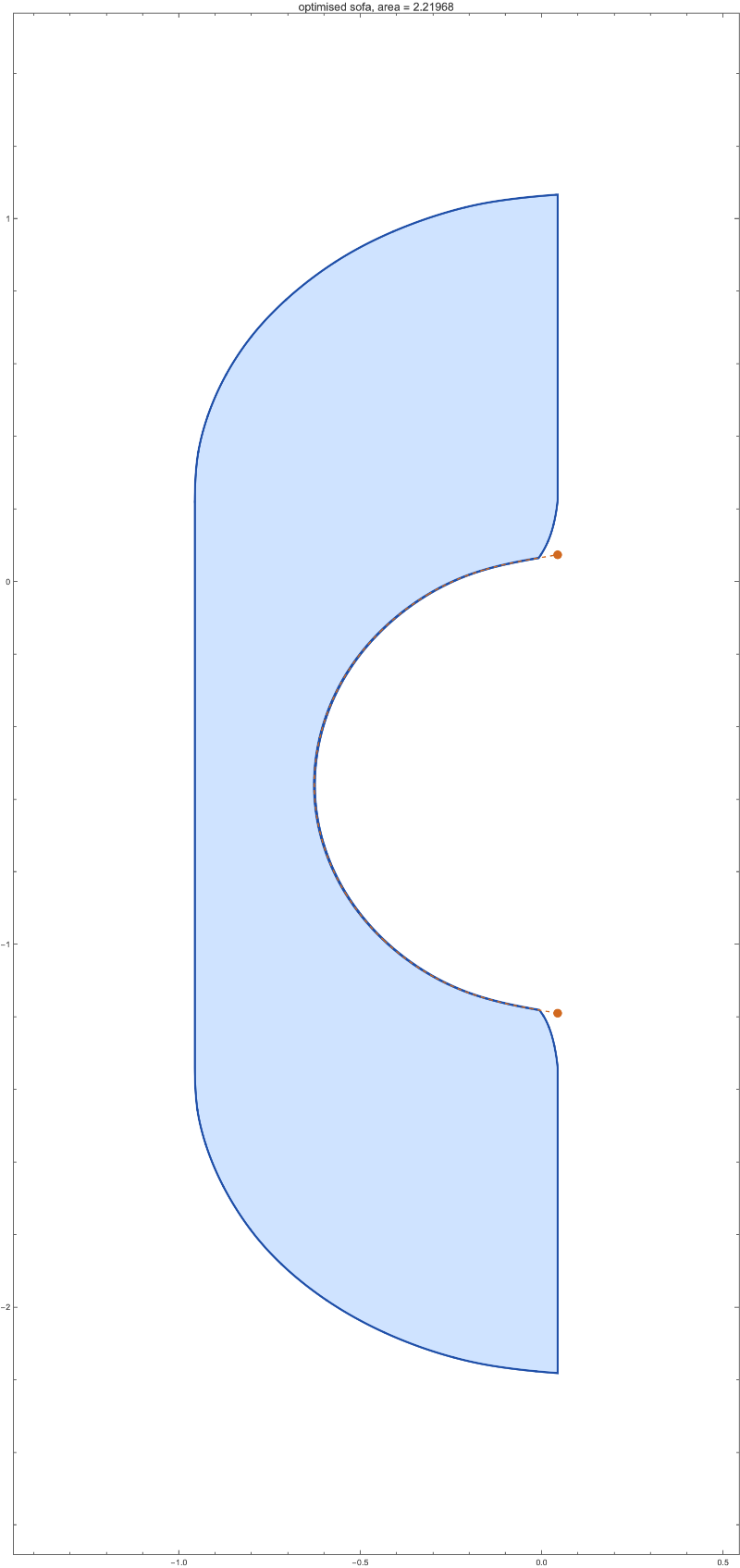
The algorithm: geometry (corridor polygons + intersections) + cubic-spline trajectory through 10 control points + Nelder–Mead with warm-started restarts. Run-time is a few minutes; the cell produces sofa.png and sofa.gif (Figures 1 and 2).

〉

import numpy as np
import matplotlib.pyplot as plt
from matplotlib.animation import FuncAnimation, PillowWriter
from matplotlib.patches import Polygon as MplPolygon
from scipy.interpolate import CubicSpline
from scipy.optimize import minimize
from shapely.geometry import Polygon, box as shp_box
from shapely.validation import make_valid

BIG = 40.0
WORLD_L = np.array([[0, 0], [BIG, 0], [BIG, 1], [1, 1], [1, BIG], [0, BIG]],
dtype=float)

def corridor(theta, cx, cy):
c, s = np.cos(theta), np.sin(theta)
ex, ey = np.array([c, -s]), np.array([s, c])
pts = np.array([cx, cy]) + (WORLD_L[:, 0:1] - 1) * ex \
+ (WORLD_L[:, 1:2] - 1) * ey
return Polygon(pts.tolist())

def build_sofa(corners, thetas):
sofa = corridor(thetas[0], *corners[0])
for i in range(1, len(thetas)):
sofa = sofa.intersection(corridor(thetas[i], *corners[i]))
if sofa.is_empty: return sofa
return sofa if sofa.is_valid else make_valid(sofa)

def trajectory(ctrl, ts):
cthetas = np.linspace(0, np.pi/2, len(ctrl))
sx = CubicSpline(cthetas, ctrl[:, 0], bc_type='natural')
sy = CubicSpline(cthetas, ctrl[:, 1], bc_type='natural')
return np.column_stack([sx(ts), sy(ts)])

def neg_area(flat, ts, M):
sofa = build_sofa(trajectory(flat.reshape(M, 2), ts), ts)
return 0.0 if sofa.is_empty else -float(sofa.area)

def quarter_arc(M, r=2/np.pi):
th = np.linspace(0, np.pi/2, M)
return np.column_stack([r * np.sin(th), r * np.cos(th)])

# Optimise
M, n_th = 10, 100
ts = np.linspace(0, np.pi/2, n_th)
x = quarter_arc(M).reshape(-1)
best = x.copy(); best_f = neg_area(x, ts, M)
print(f'initial area = {-best_f:.5f}')
for k in range(4):
init = best if k == 0 else best + 0.05 * np.random.randn(best.size)
r = minimize(neg_area, init, args=(ts, M), method='Nelder-Mead',
options=dict(maxiter=3000, xatol=1e-5, fatol=1e-7,
adaptive=True))
if r.fun < best_f: best_f, best = r.fun, r.x
print(f' round {k}: area = {-r.fun:.5f}')

# Honest area at much denser theta sampling
ts_eval = np.linspace(0, np.pi/2, 1600)
sofa = build_sofa(trajectory(best.reshape(M, 2), ts_eval), ts_eval)
print(f'\\nfinal area (1600-sample eval): {sofa.area:.5f}')

Run the cell above and you reproduce Figure 1 (the corridor sweep) and Figure 2 (the static sofa with the inner-corner trajectory).

The honest area evaluated at 1600 θ samples is 2.21968, within

2×

-4

of Gerver's bound

2.21953...

5. A literal Wolfram-Language port

The same algorithm in pure Wolfram Language. Polygon primitives carry the corridor poses and RegionIntersection composes them. The optimiser is a hand-rolled Nelder–Mead because Wolfram's FindMinimum doesn't expose Nelder–Mead and NMinimize's NelderMead path doesn't honour an initial-point seed cleanly. The three blocks below — geometry, optimiser, driver — are everything; running the driver block reproduces the Gerver-class area.

Geometry: L-corridor polygon, region intersection, spline trajectory.

A seeded Nelder–Mead in 30 lines of Wolfram.

Drive the optimisation. With M = 8 control points and 30 theta samples per call, the four warm-started rounds converge in about 100 seconds on a laptop:

Output on the machine used for this notebook:
initial area = 1.00895
round 0: area = 2.20372 (600 iters)
round 1: area = 2.24009 (600 iters)
round 2: area = 2.23959 (600 iters)
round 3: area = 2.23884 (600 iters)
honest area : 2.22195
Hammersley : 2.20742
Gerver bound: 2.21953

Once the optimiser has produced control points, the same code drives a Wolfram-native animation of the sweep:

Two equivalent ways to package the animation: ListAnimate (interactive) or Export["sofa-wolfram.gif", frames] for a portable GIF.

Scaling the angle sweep with RemoteBatchSubmit

The seven optimisations in Section 7 are embarrassingly parallel: each α is an independent Nelder–Mead run. RemoteBatchSubmit ships each anchor as a job to the Wolfram Cloud:

Each anchor takes 1–3 min, so a seven-angle sweep finishes in roughly the time of one anchor when run in parallel. Keep nRounds modest and the Wolfram Cloud compute cost stays well under a dollar.

6. Higher dimensions

The 3D set-up

A first numerical run: extruded Gerver in the tube

Build the trivial 3D construction — the 2D shape from Section 4 extruded as a unit-height prism — and slide it through the L-tube along the (lifted) 2D Gerver motion. ctrlBest is the optimised 10×2 matrix of control points from §5; the cell below picks it up directly:

7. Varying the bend angle

The seven anchor angles, side by side. Each row shows the corridor ("aisle") at that bend angle in column 2, and the optimised sofa shape (in its own frame, all drawn at the same scale) in column 3. The aisle's inner corner is marked with the orange dot.

The same data plotted as a curve, with the heuristic 1/(π - α) divergence overlaid for reference:

And finally the same family rendered as an animation — each frame interpolates the spline control points between adjacent anchor angles:

8. Summary tables

Three tables summarise what the notebook produced and how it sits in the literature: a 2D leaderboard, the 2D-vs-3D status, and the bend-angle sweep.

Table 1: 2D right-angle benchmarks

Table 2: 2D vs 3D status

Reading the table. The jump from 2D-closed to 3D-open is dramatic: a 56-year analytical effort closed the planar question, but the 3D version doesn't even have matching constructive/upper bounds with the same first digit. The cross-section shape matters a lot — square corners help, because they let the body fill the corridor's full vertical clearance regardless of horizontal position. Both 3D rows are therefore interesting open problems on their own, not just "the obvious extension".

Table 3: bend-angle sweep

References

[1] J. L. Gerver. On moving a sofa around a corner. Geom. Dedicata 42 (1992), 267–283.

[2] J. M. Hammersley. On the enfeeblement of mathematical skills by "Modern Mathematics" and by similar soft intellectual trash in schools and universities. Bull. Inst. Math. Appl. 4 (1968), 66–85. (Contains the 2.207 sofa.)

[3] Y. Kallus, D. Romik. Improved upper bounds in the moving sofa problem. Adv. Math. 340 (2018). arXiv:1706.06630.

[4] J. Baek. Optimality of Gerver's Sofa. arXiv:2411.19826 (2024).

[5] D. Romik. Differential equations and exact solutions in the moving sofa problem. Exp. Math. 26 (2017).

CITE THIS NOTEBOOK

The Moving Sofa Problem: numerical optimisation in 2D and beyond
by Marco Thiel
Wolfram Community, STAFF PICKS, May 11, 2026
https://community.wolfram.com/groups/-/m/t/3717709