Abstract
Abstract
Analyzing root networks can provide information about different characteristics of root systems, such as which properties affect each other, what the typical root network looks like, and how these properties are distributed. It also helps us identify differences between plant species that could be responsible for other phenotypic variations. In addition, creating algorithms for the digitization of paper-based botanical drawings is essential for accessing and utilizing the work done by botanists of previous decades, not to mention the wide variety of species it provides access to — many of which we have not digitized in modern formats.
Introduction
Introduction
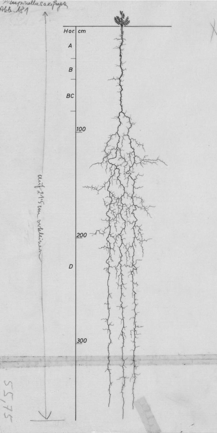
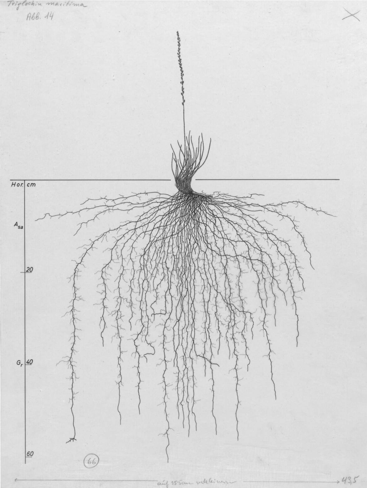
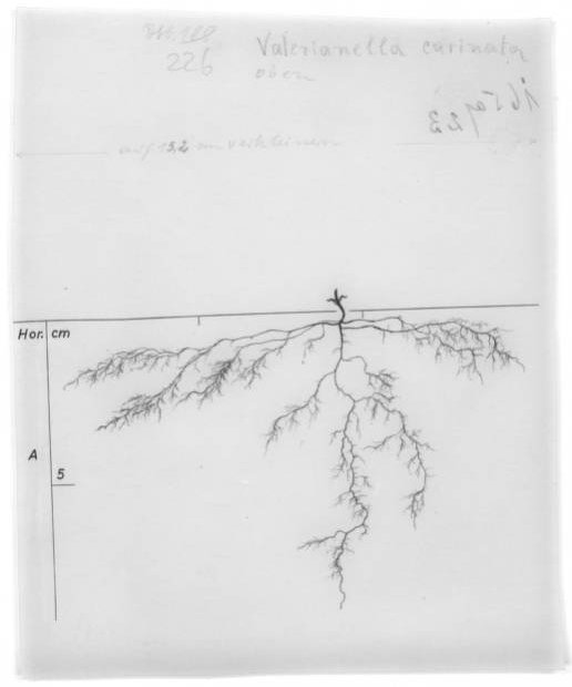
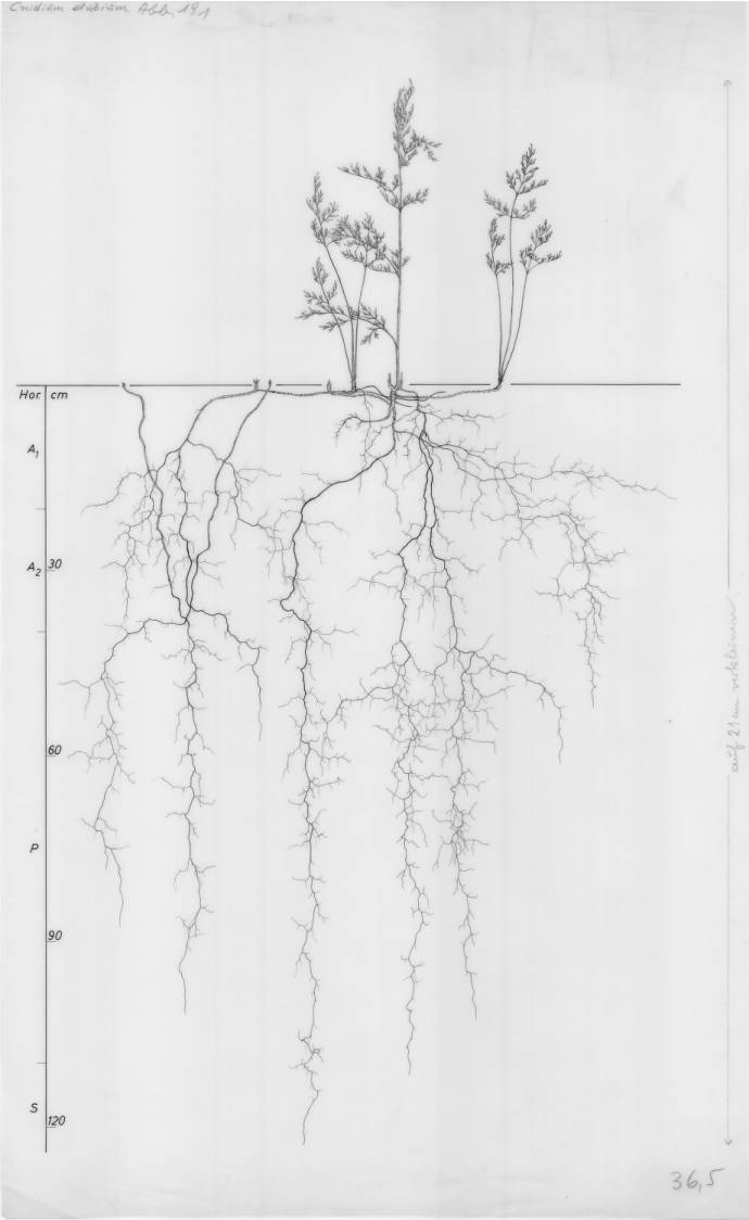
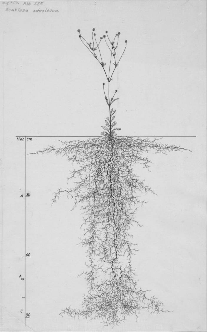
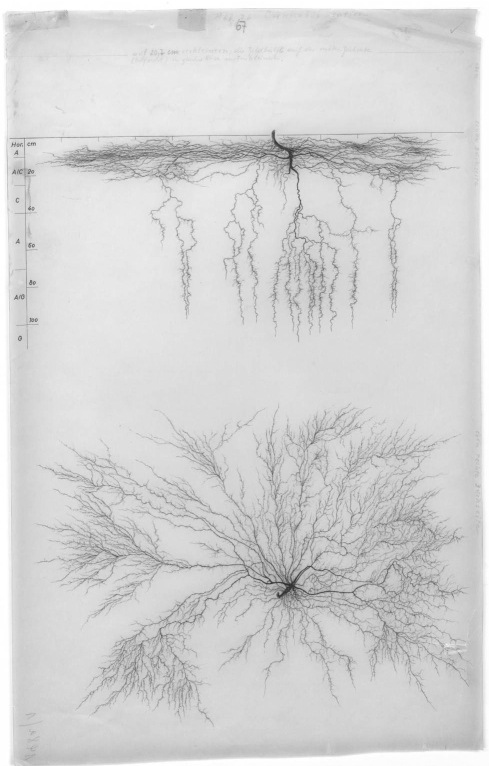
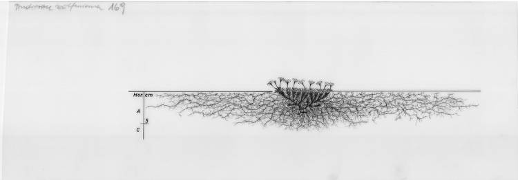
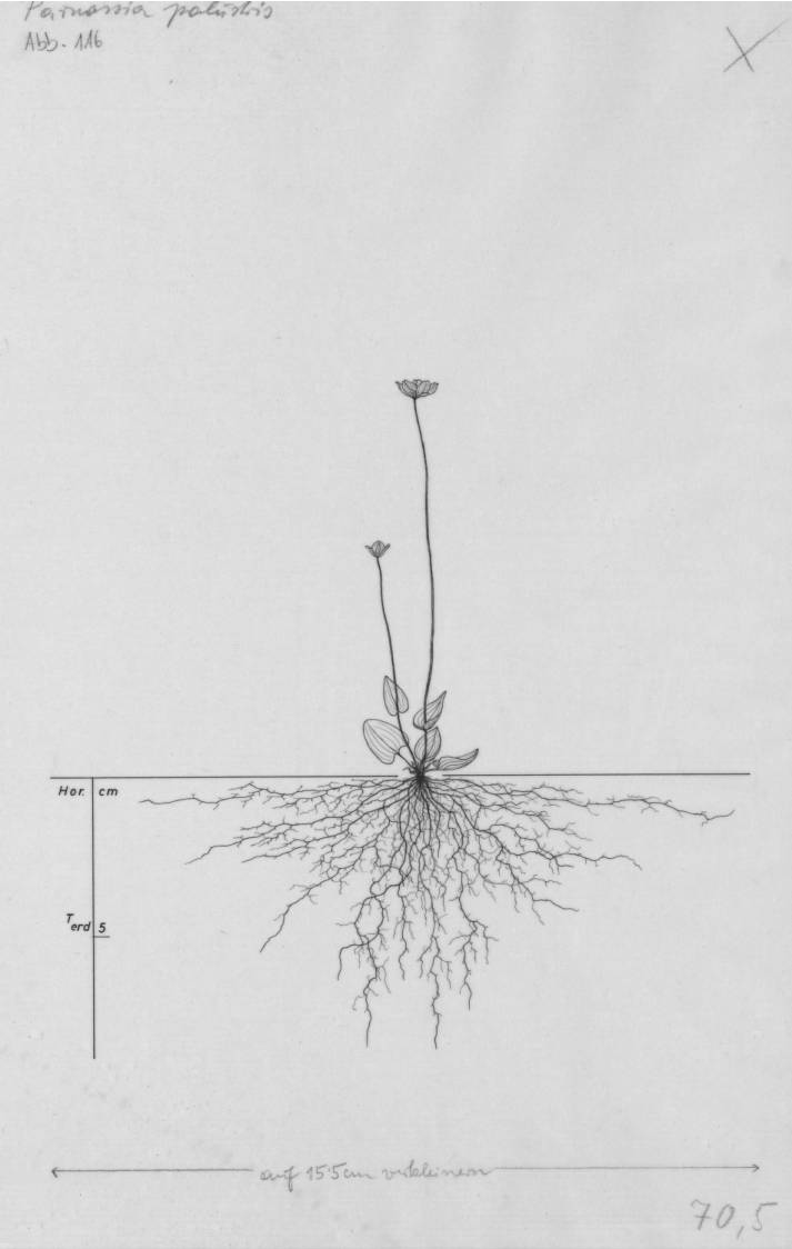
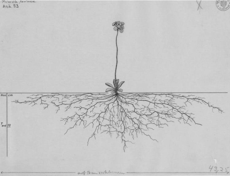
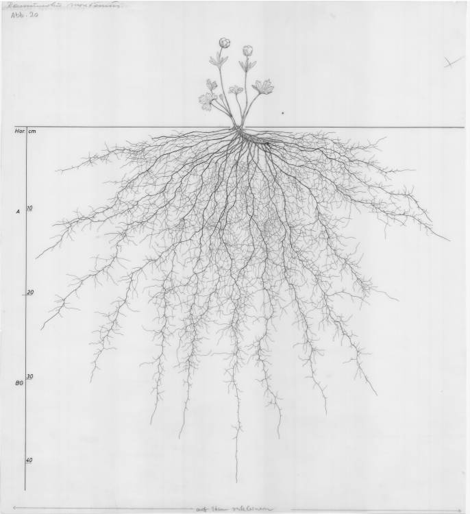
As we go about our daily lives, spent indoors more than ever, we rarely notice the wondrous array of plants that inhabit our planet. Even more rarely do we think about the surprisingly complex and beautiful world going on below the surface. My project took me exactly to this domain, exploring the characteristics of plant root networks. I worked with data provided by the University of Wageningen in the form of an online database of drawings [Wageningen]. This is an extensive collection from over 50 years of work at the university and more than a thousand catalogued species, making it ideal for observing differences in the characteristics of root networks between species [Servicedesk].
Take a look at a random sample of the dataset (the stored images have IDs ranging from 68 to 1068)
In[]:=
sampleImgList=Table[Import["https://images.wur.nl/digital/api/singleitem/image/coll13/"<>ToString[k]<>"/default.jpg"],{k,RandomChoice[Range[68,1068],10]}]
Out[]=
,
,
,
,
,
,
,
,
,
Downloading the Database
Downloading the Database
Before we can begin working we need to download the database. We also want to extract the species name from the webpages for future analysis and connect the images and the names together. If you're running this in the cloud and don't want to work with the entire dataset (which would certainly take a decent amount of both time and memory), I have also provided code for running the same functions on the sampleImgList we created earlier.
First we extract the names of the species and store them in a list
speciesList=Table[StringDrop[StringDrop[TextWords[Import["https://images.wur.nl/digital/collection/coll13/id/"<>ToString[i],"Text"]][[12]],-4],35],{i,Range[68,1068]}];
Next, we define a partitioned list to store all our IDs and loop over them 50 at a time, exporting the image to a local directory and clearing the system cache with each batch so as to not affect performance
ids=Partition[Range[68,1068],50]
Now all of the drawings are stored in the specified directory with their name being the species to which the drawing belongs.
Extracting the Root Network
Extracting the Root Network
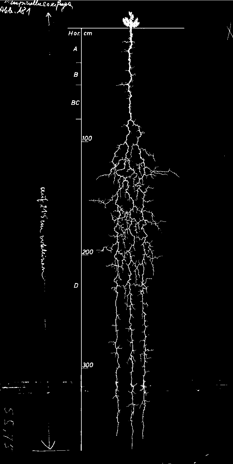
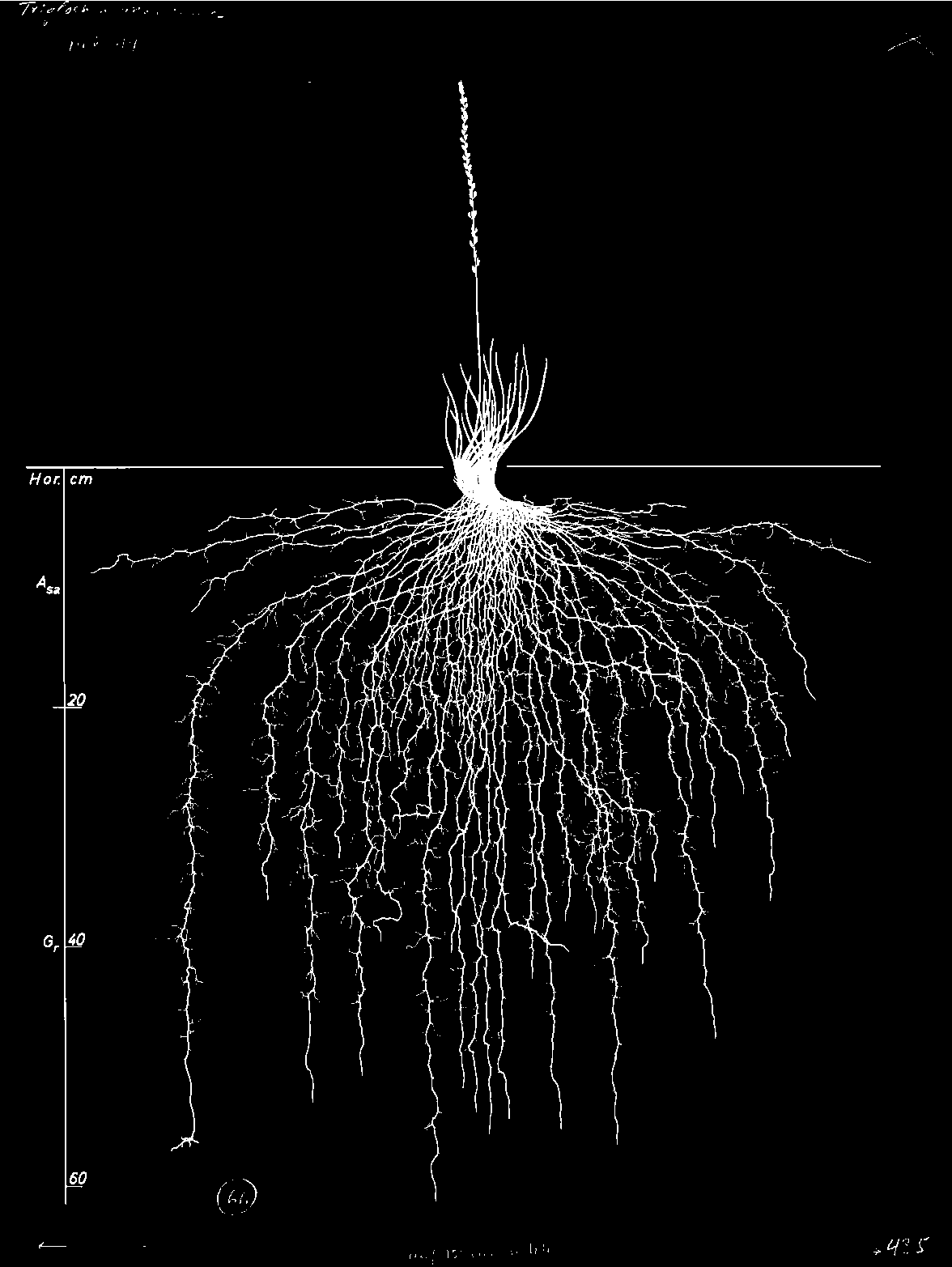
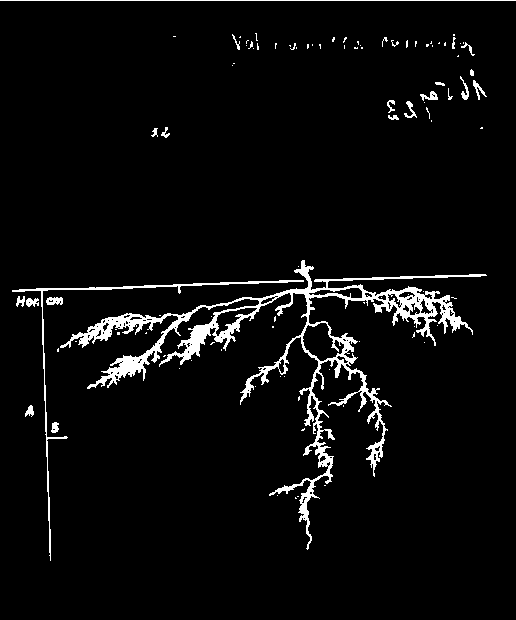
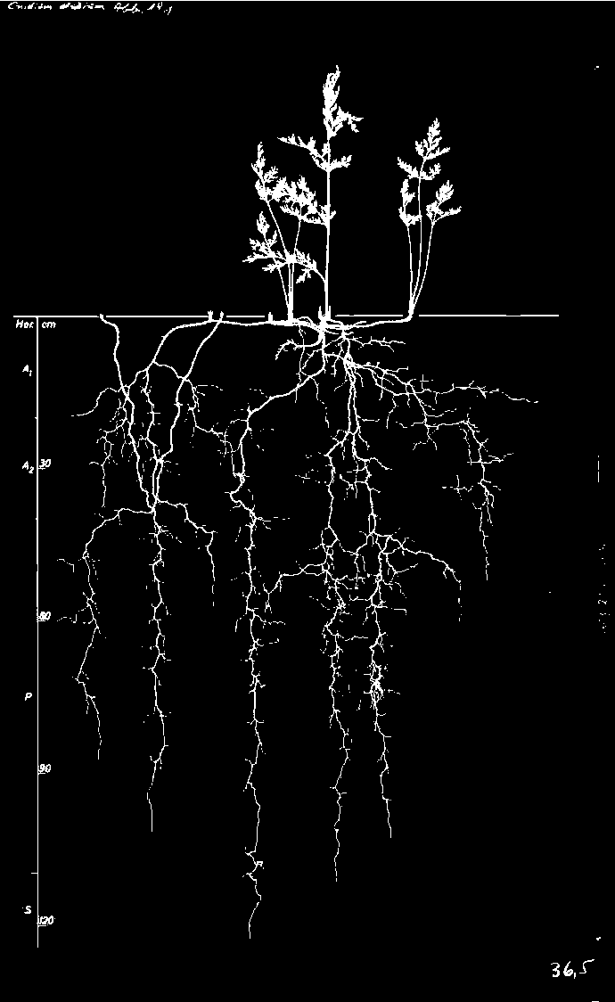
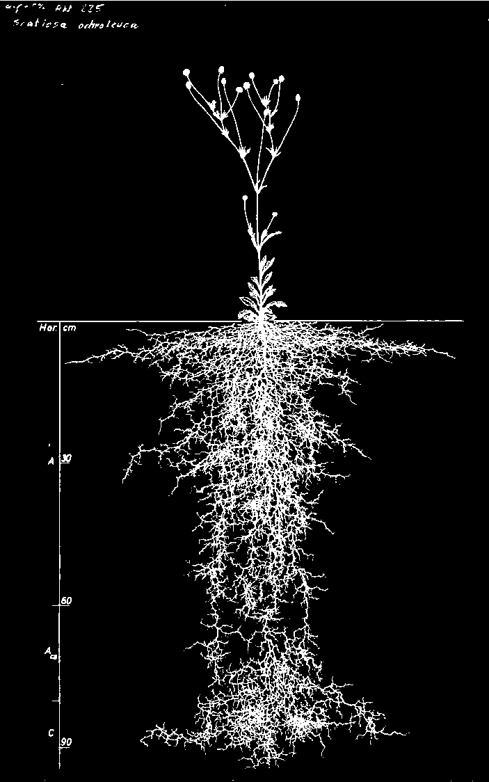
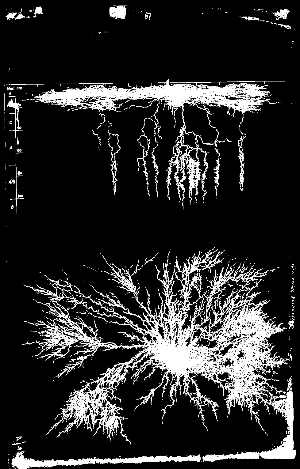
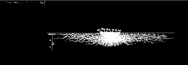
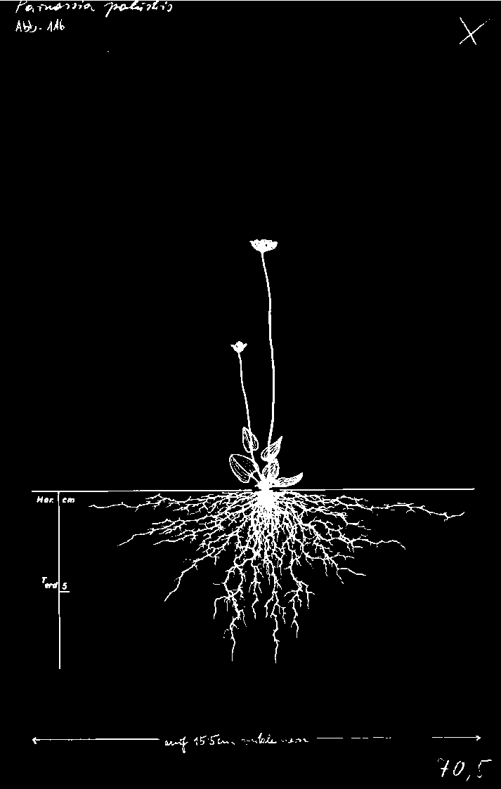
To analyze our root networks, we must isolate them from the drawing, and this is much easier said than done due to the wide variability in the drawings. Image processing is often a long game of trial and error due to the nature of working with images and the large potential for complications. Each image has 3 main parts — the root system, the shoot system and the axes and labels — with the rest being irrelevant marks like the date, catalogue number, signature of the sketcher, etc. We'll undertake the following steps, which are demonstrated on a random sample of images since performing them on all the images would take a long time (15-20 minutes/step). Binarization in particular is a critical first step in data like ours [Tensemeyer].
Binarize and ColorNegate the drawings
In[]:=
refinedSampleImgList=Table[ColorNegate@Binarize@img,{img,sampleImgList}]
Out[]=
,
,
,
,
,
,
,
,
,
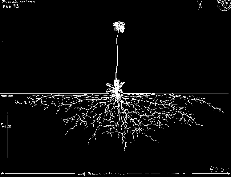
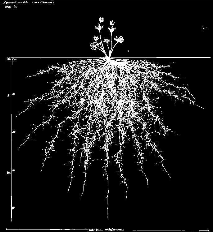
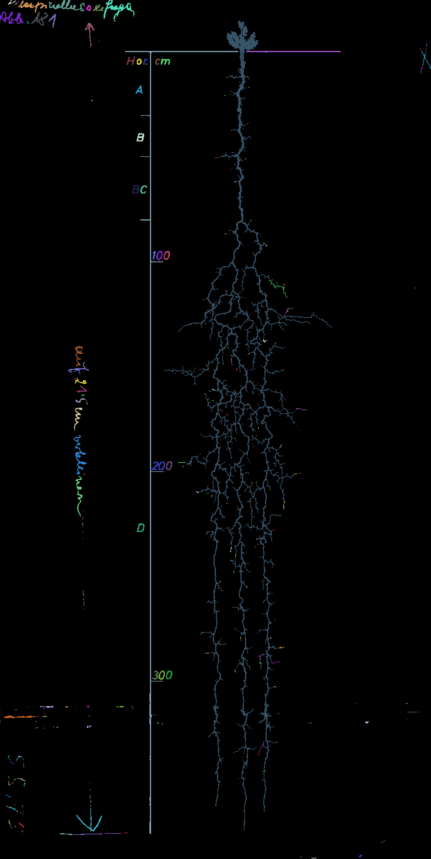
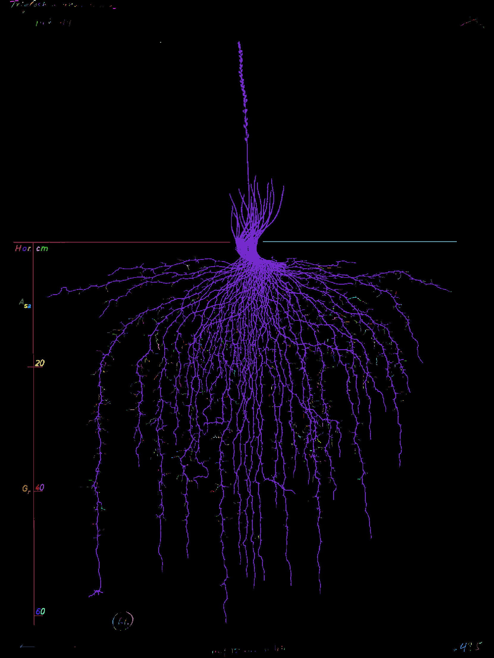
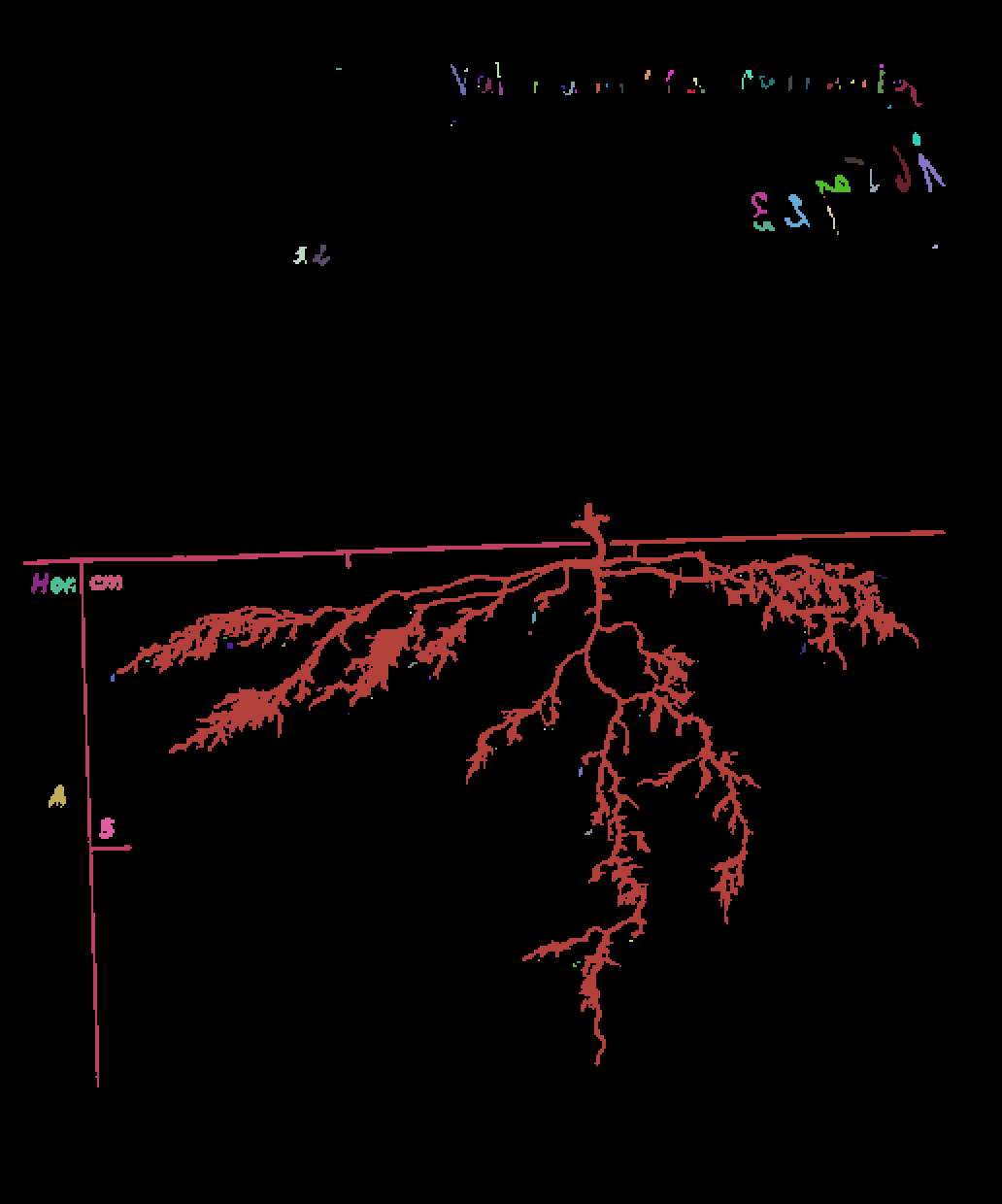
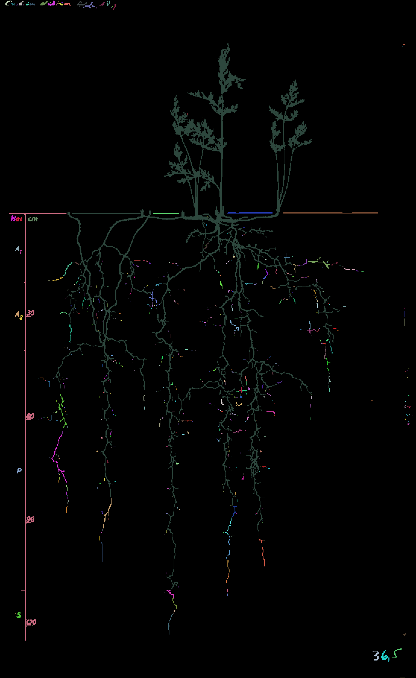
You might notice that some of the images have regions with incorrect binarization. Unfortunately this cannot be fixed since all drawings on the database are scanned uploads of physical copies. Now you might think that MorphologicalComponents[] is the logical choice for extracting the different connected components and selecting the parts we are looking for. Let's give it a go.
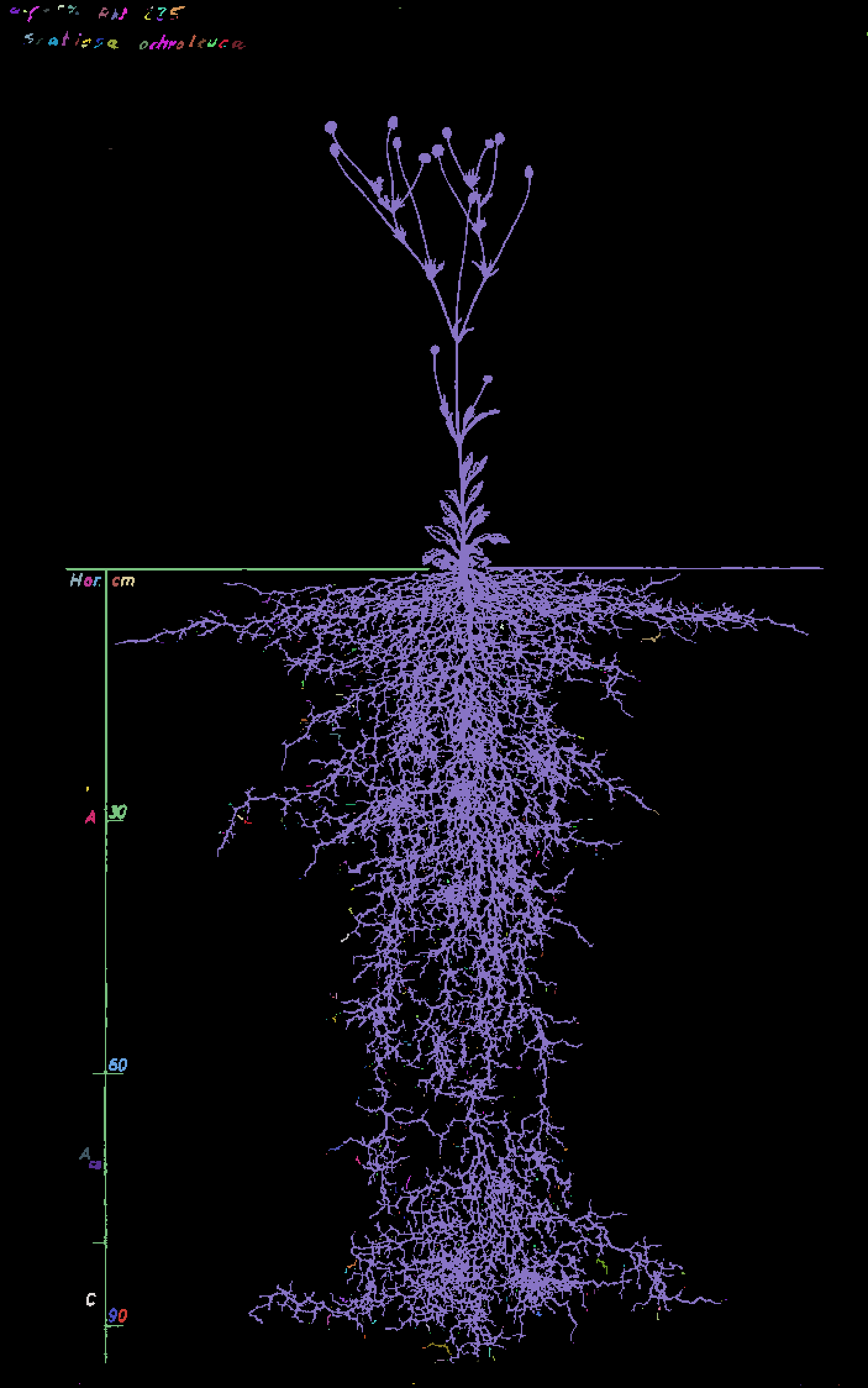
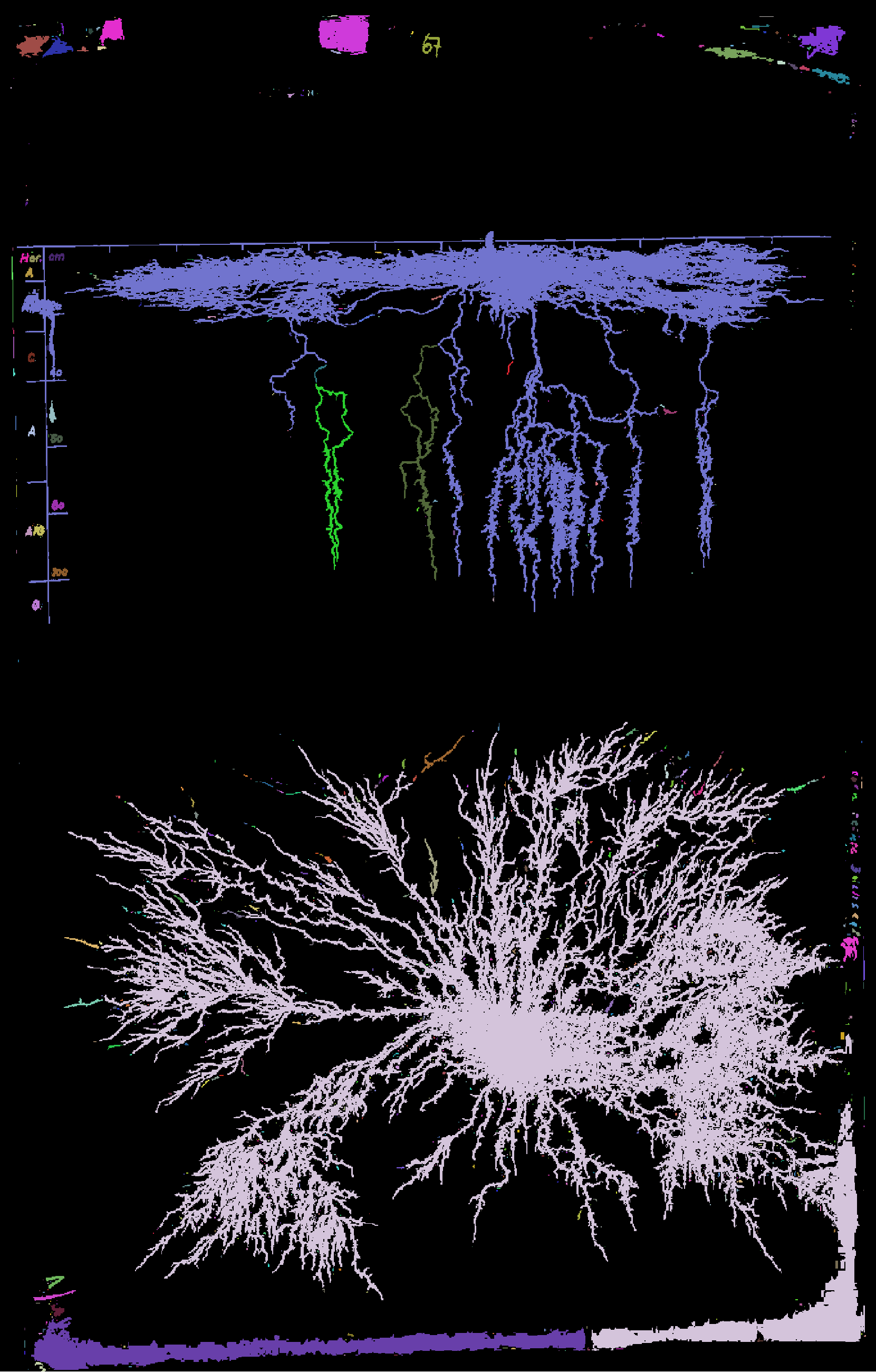
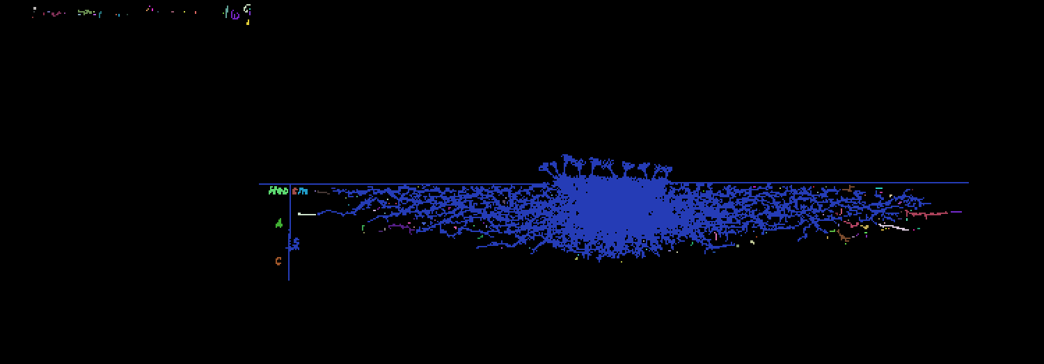
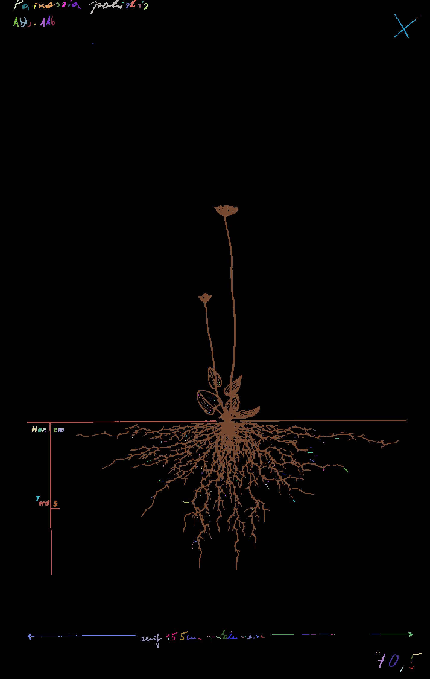
Colorized morphological components
In[]:=
Colorize[MorphologicalComponents[#]]&/@refinedSampleImgList
Out[]=
,
,
,
,
,
,
,
,
,
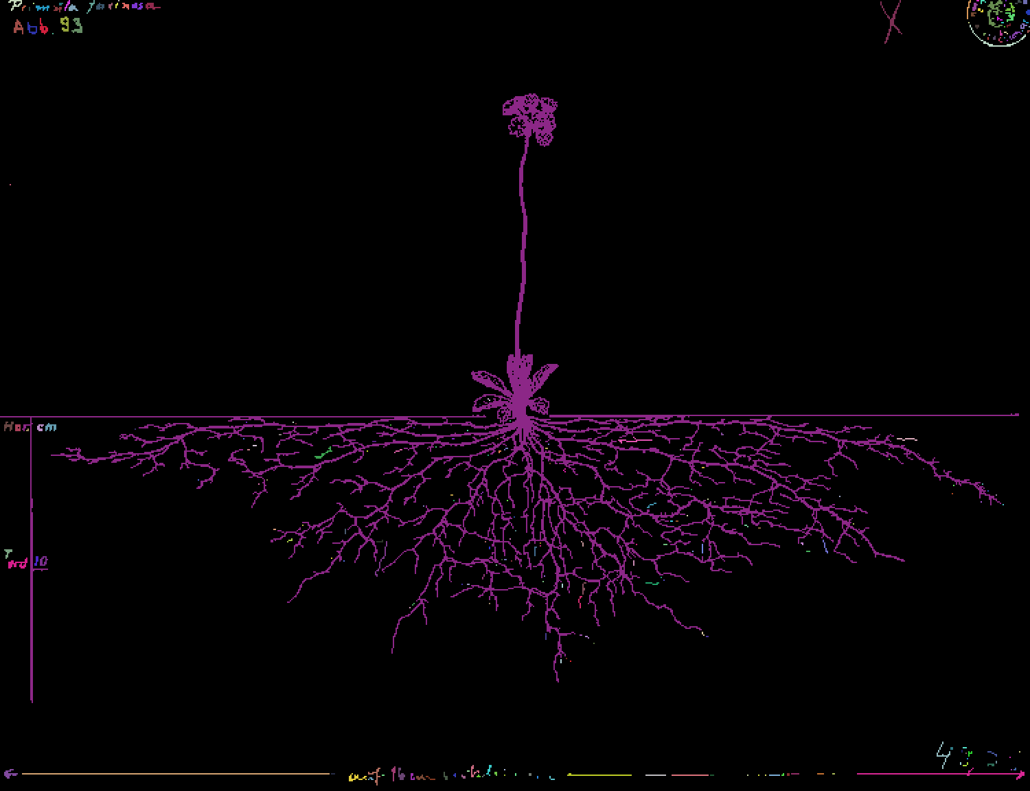
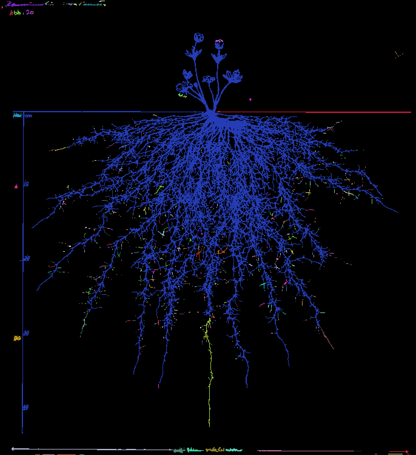
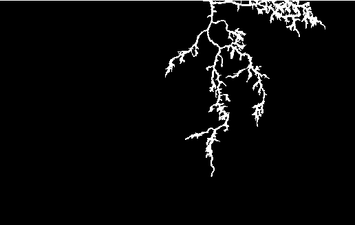
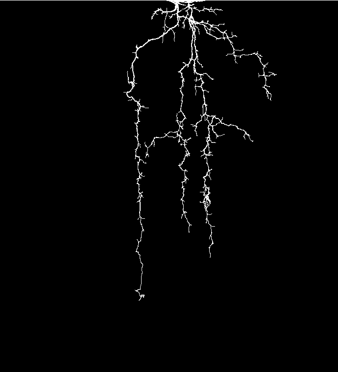
You can probably see the main problem — the shoot system and root system are part of the same morphological component. Other than that, for many drawings, the axes are also included in the same morphological component as the shoots and roots. Now we can see that our goal should be to split the images along the horizontal x-axes so we can separate the shoot from the root, and find a way to get rid of the axes and labels in the split image. A great first thought would be to use ImageLines[], since it is designed to recognize lines in images, but upon testing it we find out that it finds huge numbers of lines and its strongest lines are not even on the axes! To get around this, we write our own function.
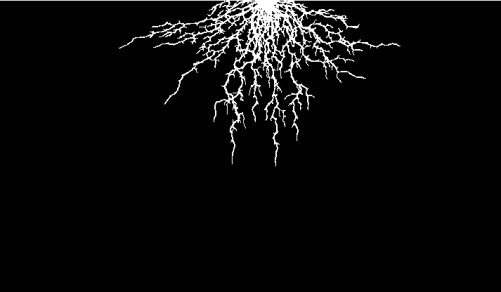
Customized function to split images
In[]:=
cropDrawing[img_]:=Quiet@Module[{coordsList,slopeList,indexMinSlopes,distFromCenterList,finalMinIndex,nimg=ColorNegate@Binarize@img},coordsList=ImageLines[nimg,0.2][[All,1]];slopeList=Abs@Map[#[[2]]/#[[1]]&,#[[2]]-#[[1]]&/@coordsList];indexMinSlopes=Flatten[Position[slopeList,#]&/@Select[slopeList,#<1&]];distFromCenterList=Total/@Abs[coordsList[[indexMinSlopes,{1,-1},-1]]-.8Last@ImageDimensions[nimg]];finalMinIndex=indexMinSlopes[[Flatten[Position[distFromCenterList,Min@distFromCenterList]][[1]]]];SelectComponents[ImageTake[nimg,(-coordsList[[finalMinIndex,-1,-1]]-coordsList[[finalMinIndex,1,-1]])/2+10],"Count",-1]]cropDrawing[#]&/@sampleImgList
Out[]=
,
,
,
,
,
,
,

,
,
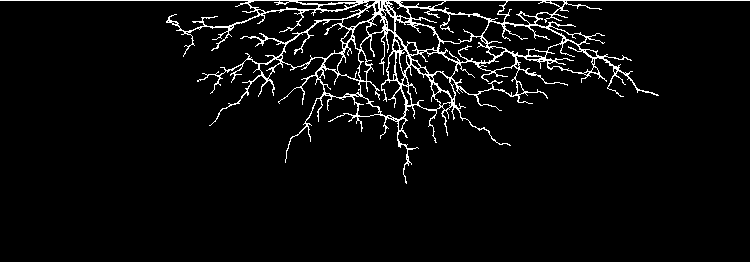
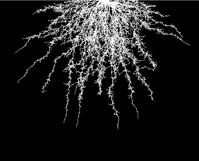
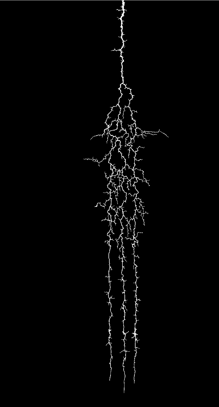
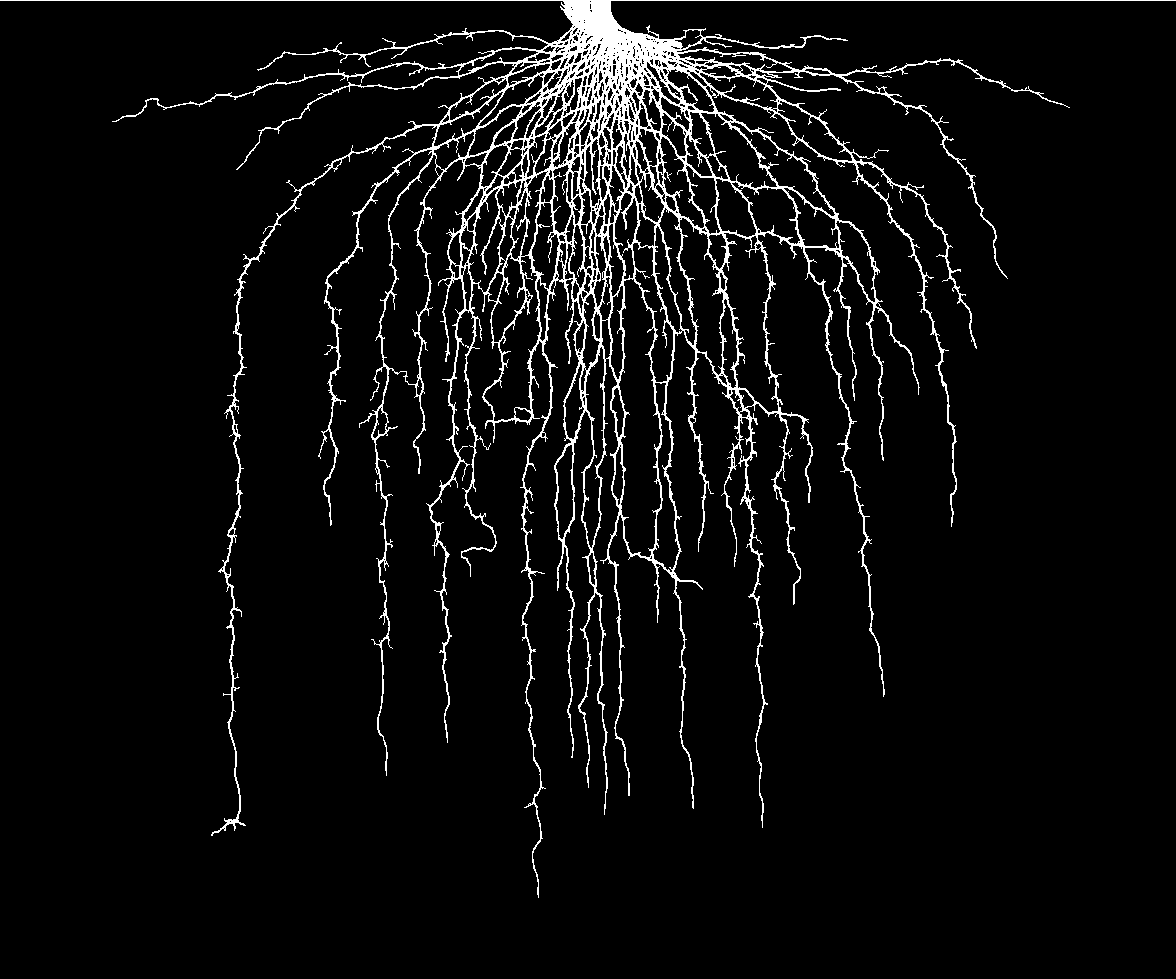
In a nutshell, the function cropDrawing[] takes an image and then applies the following steps in order:
◼
Uses ImageLines[] with a threshold of 0.2 and stores the coordinates in a new list
◼
Calculates the slope of each of the lines
◼
Discards lines with a slope larger than 1
◼
For the remaining lines, calculates the distance from four-fifths of the way up the image
◼
Selects the line with the smallest distance
◼
Crops the image at a line 10 pixels below the line determined in the previous step
◼
A vertical shift of 10 helps eliminate the axes from the vast majority of images which would otherwise not have been possible to remove
Processing the entire batch of downloaded images
Not all of the images will be successfully cropped. Out of the full dataset of a 1000+ images, there are ~20 tilted drawings, made on an axis that is at an angle to the horizontal. ~30 images are also double/triple ones, where the same drawing has multiple views (top/side/etc.). And lastly, ~70 images were incorrectly binarized, which, again, isn't something we can work around. For the titled and double/triple drawings, we technically could modify our algorithm to include them, but that would make it much more complex and take a good amount of time to do. The law of diminishing results applies here [Brittanica]. Of the remaining images, the algorithm failed on only 11% of them, which is a very high success rate! At this point, though, you'll have to go into the directory where the images have been exported and manually remove the ones that fit into one of the above categories, or you could crop the root networks which only had slight deficiencies, which is what I did. When this is done, we'll have a final, processed dataset and we can move on to actually measuring the characteristics and analyzing the roots.
Measuring Root Characteristics
Measuring Root Characteristics
Given below is a list of the properties that we will be measuring [Wolfram].
◼
Area: the area occupied by the root network
◼
PerimeterLength: the length of its perimeter
◼
MaxPerimeterDistance: the maximum distance of any point on the root network from the perimeter
◼
Centroid: the coordinates of the centroid
◼
Medoid: the coordinates of the medoid
◼
MeanCentroidDistance: the average distance to the centroid
◼
MaxCentroidDistance: the maximum distance of any point to the centroid
◼
MinCentroidDistance: the minimum distance of any point to the centroid
◼
Orientation: the angle between the largest axis and horizontal axis of the best-fitting ellipse
◼
Elongation: (1 - width/height) of the oriented best-fit ellipse
◼
Eccentricity: the eccentricity of the oriented best-fit ellipse
◼
Circularity: 2πr/p where r is the equivalent disk radius ‘r’ and polygonal length ‘p’
◼
BoundingBox: coordinates of the bounding box
◼
BoundingBoxArea: area enclosed by the bounding box
◼
MinimalBoundingBox: smallest possible oriented bounding box
◼
Rectangularity: Fraction of pixels within the minimal bounding box
◼
BoundingDiskCenter: coordinates of the center of the bounding disk
◼
BoundingDiskRadius: radius of the bounding disk
◼
BoundingDiskCoverage: coverage of bounding disk area by the root network area
◼
ConvexVertices: corner elements of the convex hull
◼
ConvexArea: area of the convex hull polygon
◼
ConvexPerimeterLength: length of the convex hull polygon's perimeter
Defining the list:
Now we need a function that will calculate all of these for us, something that we can loop over our images of root networks
Function to get root network properties
As always, we’ll loop over the images 25 at a time and get their properties, then store the properties in an association with the keys being the species name for easy retrieval. We do need to declare imgNameList and partImgNameList since we removed improper images and so the list of species in our data has changed. Once this is done we'll have an association of associations that is easily slice-able.
Creation of the main dataset
Other than the properties listed above, we'll also calculate the number of branch points, i.e. how many times the root network splits/branches out, and append this to our dataset.
Now we'll create a new association that organizes everything by the property name, since that is what primarily matters during our analysis.
Creating our association:
Analyzing Root Characteristics
Analyzing Root Characteristics
We have all the data; it's time to see what interesting relationships and patterns we uncover! If you haven't been running the image processing steps on the entire dataset (fair enough, that would take 30 minutes at a minimum) then you can also use the code below to import the final dataset of image properties into the variable propertyValsByProp that we're going to be using for analysis. For our analysis we are also defining a new list called numericalProperties since many of the properties we were measuring (e.g. Centroid, BoundingBox, etc.) are coordinates of positions instead of numbers whose distributions we can plot.
Defining a new list of numerical properties
Importing final dataset of characteristics
Create histograms to visualize property distributions
That is a lot of data! We can see that most of the distributions have a relatively low mean and are heavily right-skewed. Elongation seems to be much more consistent across the board and the eccentricity is actually left-skewed. Let's calculate some important statistical measures so we can quantify the trends we observe. We're also going to rescale the data to be between 0 and 1 because they have vastly different ranges, which would make their unnormalized calculations much harder to compare [COS436].
Calculating 5 statistical measures and displaying them in a grid
Again, this re-affirms what we observed with the histograms. Kurtosis is really interesting, as it is a measure of the combined weight of a distribution’s tails relative to the center of the distribution. Excess kurtosis, defined as (kurtosis - 3) tells us whether the data is leptokurtic (excess kurtosis > 0), mesokurtic (excess kurtosis = 0) or platykurtic (excess kurtosis < 0). A leptokurtic distribution is skinny, with long tails because of outliers. On the other hand, a platykurtic distribution is broad and flatter. Lastly, a mesokurtic distribution has the same kurtosis as the normal distribution [Kenton].
In the data here, MinCentroidDistance seems to have lowest mean and median, which means that most of its values are very strongly clustered but there are a bunch of outliers which stretch out the range, and indeed that is what we observe; one observation greater than 100 is significantly distorting the scale, which also gives it gigantic skewness and kurtosis values. Orientation, eccentricity and especially elongation are pretty close to the normal distribution's skewness of 0, and eccentricity also happens to be almost mesokurtic. If we need to calculate the probabilities that certain plant root networks will have a certain value for a characteristic, we can use PDFs or probability distribution functions.
In the data here, MinCentroidDistance seems to have lowest mean and median, which means that most of its values are very strongly clustered but there are a bunch of outliers which stretch out the range, and indeed that is what we observe; one observation greater than 100 is significantly distorting the scale, which also gives it gigantic skewness and kurtosis values. Orientation, eccentricity and especially elongation are pretty close to the normal distribution's skewness of 0, and eccentricity also happens to be almost mesokurtic. If we need to calculate the probabilities that certain plant root networks will have a certain value for a characteristic, we can use PDFs or probability distribution functions.
Fitting PDFs to each property's distribution
Moving on, we'll calculate the correlations between the different properties, which might be even more interesting than the distributions. The exact measure we are using is Pearson's Correlation Coefficient, which measures linear correlations [Kent State].
Create a function that provides the correlation between two properties
Let's create a matrix to easily glean information. In the heatmap below, a red color represents a perfect positive correlation and a blue color represents a perfect negative correlation, with the spectrum in between running between 1 and -1.
First off, the diagonal, of course, has perfect 1-to-1 correlations, since we're calculating the correlations between the same properties. We do have many other interesting correlations to look at.
◼
Area and PerimeterLength have a really strong correlation, telling us that as a root network’s perimeter increases, its area tends to do the same. Thus there aren’t many root shapes with a high area but low perimeter (i.e. circular) which is reasonable as roots would tend to branch out.
◼
Area and PerimeterLength also have strong correlations with BoundingBoxArea, BoundingDiskRadius, ConvexArea and ConvexPerimeterLength, all of which is expected. Their extremely strong linear correlation with BranchPoints, though, informs us that roots branch at a relatively consistent rate as the network systems get bigger.
◼
MaxPerimeterDistance isn't strongly correlated with anything. In a way, MaxPerimeterDistance is a measure of how "bunched up" the roots are, so that quantity apparently isn't correlated that highly with any characteristic.
◼
MaxCentroidDistance and MeanCentroidDistance also have a surprisingly high correlation, which is unexpected because there is nothing to suggest that the farthest point in the network should have anything to do with the average point. What this tells us is that root networks branch out in roughly-equal branches lengthwise, so there aren't any branches that are much longer than the other ones. Both of them are also strongly correlated with ConvexPerimeterLength, ConvexArea, BoundingBoxArea, and Area and PerimeterLength in general, which makes logical sense since all of these values are indirectly related to the root network's size.
◼
MinCentroidDistance isn't correlated much with any property either, and in fact much of it, according to the histogram, is very close to 0 in general.
◼
Orientation has pretty low correlation coefficients as well.
◼
Elongation and Eccentricity have really high correlations, which makes sense as they are both measuring very similar qualities in the root networks.
◼
Circularity seems to be negatively correlated with a lot of properties and looking at the scatterplots reveals an inverse square relationship. In general, as roots develop and grow, they become less and less circular since they want to maximize their surface area for collecting water/nutrients (i.e.) their perimeter and minimize the size of these branches (i.e. area), while a circle does the exact opposite.
◼
Rectangularity has a decently strong correlation with BoundingDiskCoverage, but not much else. Both of them are measures of component area divided by the total area of the bounding box and bounding disk respectively, so this correlation is explainable, but still interesting nonetheless, since it implies that root networks that fit nicely into rectangles also fit nicely into circles, which isn't immediately obvious. Again, as networks grow, they tend to branch out and deviate from both of these shapes.
◼
There are a few other expected correlations (like BoundingBoxArea with ConvexArea, ConvexArea with ConvexPerimeterLength, etc.) but the strong correlations between BranchPoints and many of the other properties is striking, and indicates that it's connected not only to the expected Area and PerimeterLength, but also to things like the MaxCentroidDistance and BoundingBoxArea. This is a symptom of the fact that a number of properties turned out to be more interconnected that presumed, such as BoundingBoxArea and PerimeterLength.
The line below generates a grid of plots of points between all the different characteristics
If you're interested, you can use the functions below to see which specific root networks possess the largest and/or smallest values for a particular property.
Computational Art
Computational Art
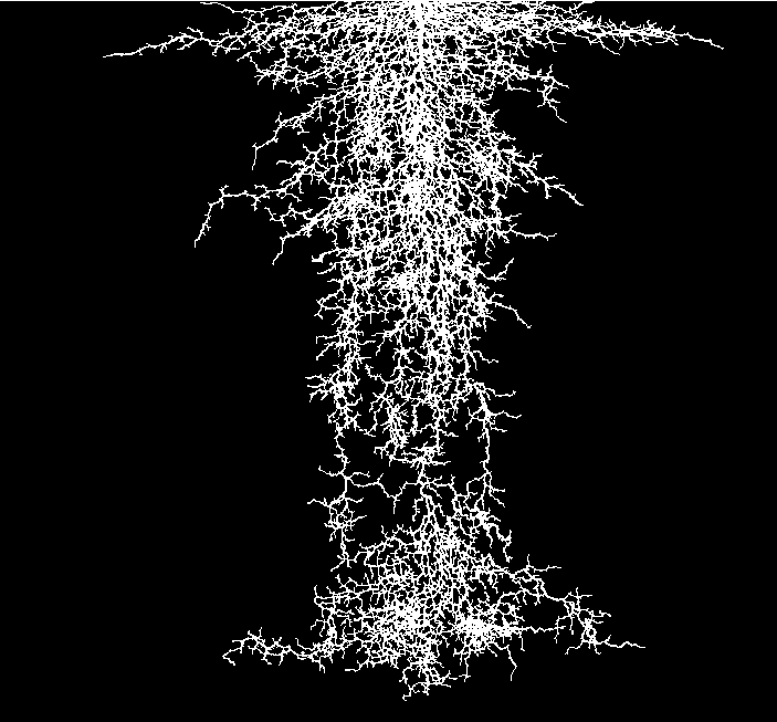
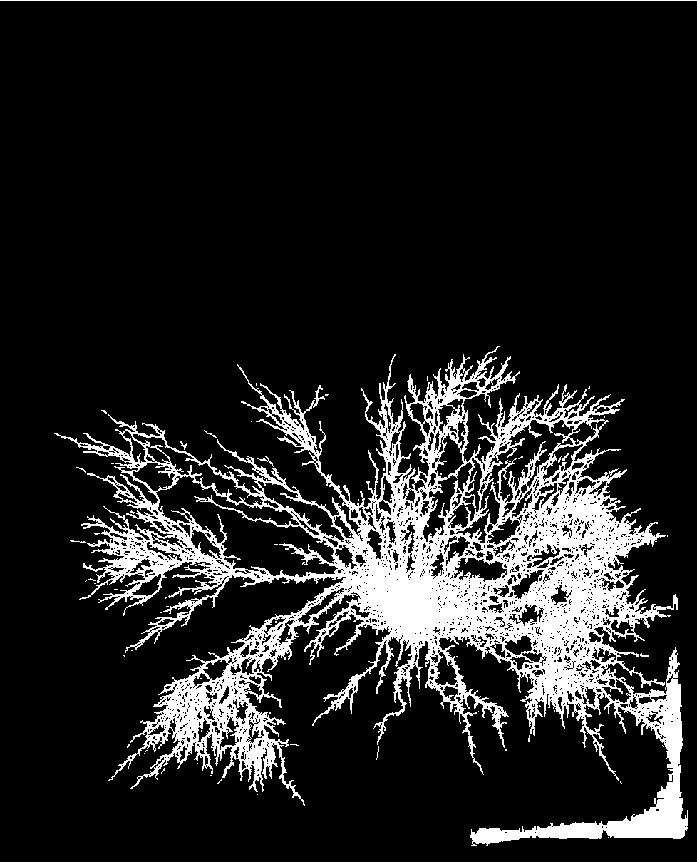
Believe it or not, root systems can actually be used to create some amazing computational art! I stumbled upon this while playing around with the image processing functions. Feel free to use the function below to generate your own, and do visit the gallery at https://plantrootart.tumblr.com/ for viewing all the computational art that this project created.
Conclusion
Conclusion
Computational botany is still a relatively unexplored field, but one that has the potential to drastically increase the amount of information we have about plants and the research we can perform on that data, similar to how computers have spurred advances in other fields in the life sciences. The large number of samples from a range of different species has offered insights into a much larger section of the plant world than focusing on specific families would have. The new algorithm developed for image processing here also makes the Wageningen University's vast database accessible to future researchers. And of course, the computational art is a nice touch to round the project out.
References
References
[Kent State] Kent State University. “SPSS Tutorials: Pearson Correlation.” LibGuides, 8 July 2021, libguides.library.kent.edu/SPSS/PearsonCorr.
[Kenton] Kenton, Will. “Kurtosis.” Investopedia, Nov. 2020, www.investopedia.com/terms/k/kurtosis.asp.
[COS436] Princeton COS436. “Scaling.” Princeton University, 2008, www.cs.princeton.edu/courses/archive/fall08/cos436/Duda/PR_Mahal/scaling.htm.
[Servicedesk] Servicedesk Library. “Drawings of Root Systems in Image Collections.” WUR, 11 Apr. 2017, www.wur.nl/en/newsarticle/Drawings-of-Root-Systems-in-Image-Collections.htm.
[Tensemeyer] Tensmeyer, Chris, and Tony Martinez. “Historical Document Image Binarization: A Review.” SN Computer Science, vol. 1, no. 3, 2020. Crossref, doi:10.1007/s42979-020-00176-1.
[Brittanica] The Editors of Encyclopaedia Britannica. “Diminishing Returns | Definition & Example.” Encyclopedia Britannica, 27 Dec. 2017, www.britannica.com/topic/diminishing-returns.
[Wageningen] Wageningen University. “Root System Drawings.” Wageningen University & Research, 2017, https://images.wur.nl/digital/collection/coll13/search/page/1.
[Wolfram] Wolfram Research, Inc. “ComponentMeasurements—Wolfram Language Documentation.” Wolfram Documentation Center, Wolfram Research, Inc., https://reference.wolfram.com/language/ref/ComponentMeasurements.html. Accessed 15 July 2021.
[Kenton] Kenton, Will. “Kurtosis.” Investopedia, Nov. 2020, www.investopedia.com/terms/k/kurtosis.asp.
[COS436] Princeton COS436. “Scaling.” Princeton University, 2008, www.cs.princeton.edu/courses/archive/fall08/cos436/Duda/PR_Mahal/scaling.htm.
[Servicedesk] Servicedesk Library. “Drawings of Root Systems in Image Collections.” WUR, 11 Apr. 2017, www.wur.nl/en/newsarticle/Drawings-of-Root-Systems-in-Image-Collections.htm.
[Tensemeyer] Tensmeyer, Chris, and Tony Martinez. “Historical Document Image Binarization: A Review.” SN Computer Science, vol. 1, no. 3, 2020. Crossref, doi:10.1007/s42979-020-00176-1.
[Brittanica] The Editors of Encyclopaedia Britannica. “Diminishing Returns | Definition & Example.” Encyclopedia Britannica, 27 Dec. 2017, www.britannica.com/topic/diminishing-returns.
[Wageningen] Wageningen University. “Root System Drawings.” Wageningen University & Research, 2017, https://images.wur.nl/digital/collection/coll13/search/page/1.
[Wolfram] Wolfram Research, Inc. “ComponentMeasurements—Wolfram Language Documentation.” Wolfram Documentation Center, Wolfram Research, Inc., https://reference.wolfram.com/language/ref/ComponentMeasurements.html. Accessed 15 July 2021.