In this notebook, we derive the Riemann curvature tensor in the calculus from the commutator of covariant derivatives applied to a vector field in . eliminates the tiresome, hazardous manual checking of indices and algebraic signs that every physicist has experienced. automates covariant differentiation, tensor quotienting, canonicalizing indices, etc.
μ
A
In addition, this notebook demonstrates translating the expressions into calls of MetricTensor and ChristoffelSymbol from the Wolfram Function Repository (WFR). A proof-of-concept compiler backend performs this lowering. We plan to further develop this compiler in future versions to bridge the labor-saving benefits of to established tools in Wolfram and the WFR.
This notebook is an occasion for a major, non-breaking refactoring of over previous versions. The code still runs all the old tests and reproduces all the old results.
◼
A .wl block-version of code for this notebook, minus the prose and the compiler POC, is available at https://github.com/rebcabin/RelativityToolkit/blob/main/calculate_riemann.wl.
Initialize the Relativity Toolkit
Initialize the Relativity Toolkit
Optional: Quit for a Fresh Kernel
Optional: Quit for a Fresh Kernel
◼
Note, if you call Quit in a notebook, evaluation may hang. If you want to “Evaluate Notebook,” mark the following cell “Evaluatable” in the CellProperty menu, call Quit once, then comment out the Quit cell, or mark it unevaluatable again. Alternatively, you can quit the kernel via the Evaluation menu (last item). At that point, you can “Evaluate Notebook” in a clean environment. Otherwise, you can evaluate cells in this notebook individually.
->
(*CellisnotEvaluatablebydefault*)Quit[];
Download the Code
Download the Code
In[]:=
RTbranch="main";RTbase="https://raw.githubusercontent.com/rebcabin/RelativityToolkit/"<>RTbranch<>"/";RTbust="?t="<>ToString[Round[AbsoluteTime[]]];(*Forcefreshdownload*)RTrules=RTbase<>"RelativityToolkit.wl"<>RTbust;RTtests=RTbase<>"RelativityToolkit_RegressionTests.wl"<>RTbust;RTviz=RTbase<>"RelativityToolkit_VisualShowcase.wl"<>RTbust;Get[RTrules];
»
Relativity Toolkit version :1.8.0
»
Relativity Connection Symbol :Γ
Optional: See all Tests and Results from Prior Works
Optional: See all Tests and Results from Prior Works
Make any of the following cells evaluatable if you wish. They’re unevaluatable by default to keep this notebook trim.
Get[RTtests];
In[]:=
Get[RTviz](*nosemicolon,onpurpose*)
In[]:=
Get[RTbase<>"covariant_derivative.wl"]
In[]:=
Get[RTbase<>"law_of_gamma.wl"]
In[]:=
Get[RTbase<>"connections_to_christoffels.wl"]
Configure Relativity Connection Symbol
Configure Relativity Connection Symbol
To properly compose covariant derivatives, must know the user’s reserved symbols for non-tensorial connection coefficients. In gravitational physics, these force-producing connections are called Γ (capital gamma). Other theories like electrodynamics and Yang-Mills that can benefit from use other connection symbols.
We’re going with Γ for this relativity/gravitation notebook.
In[]:=
SetConnection[Γ];
Relativity Engine: Connection set to Γ
The Geometric Definition
The Geometric Definition
Misner, Thorne, & Wheeler [MTW] start in Box 11.5, page 265, with a commutator of covariant derivatives:
In[]:=
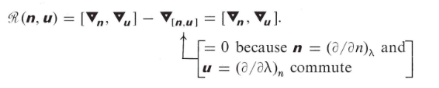
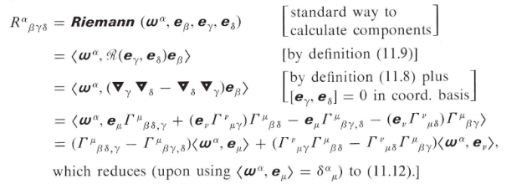
then they derive a component representation, Equation 11.12, in Exercise 11.3, page 276:
The Derivation in Index Notation
The Derivation in Index Notation
MTW’s geometric forms are too high-level for . The index notation is just right. Let’s start with the commutator
Step 1: Formulate and Differentiate
Step 1: Formulate and Differentiate
First, remind ourselves of the action of our covariant derivative, CD, trusted from earlier notebooks and tests. Apply CD to a concrete contravariant vector, in lieu of MTW’s abstract basis forms:
β
A
In[]:=
EchoCD[A[[α]],x[[δ]]]," ≡ =";
∇
δ
β
A
β
A
;δ
»
∇
δ
β
A
β
A
;δ
A
α
,δ
λ11
α
Γ
δλ11
◼
Note the generated summation index. keeps track of such and prevents cross-capture with meaningful (free) indices in big calculations.
◼
TODO: we might add basis abstractions to a future version of . It’s lower priority, however, as we get the same results by application of Quotient Theorems.
The commutator applies another covariant derivative, as in , then reverses the order of γ and δ and subtracts: -. However, composing covariant derivatives blindly conceals a trap: the product rule of CD only pertains to products of tensors, but the inner CD produces products like , a tensor times a non-tensor! The next section introduces the fix:
∇
γ
∇
δ
β
A
∇
γ
∇
δ
β
A
∇
δ
∇
γ
β
A
A.Γ
Boxing Non-Tensorial Terms
Boxing Non-Tensorial Terms
When we apply the “outer” to the “inner” , CD must treat the “inner” =- as a whole tensor. That means CD must not apply the ∇ product rule to the term .
∇
γ
∇
δ
β
A
∇
δ
β
A
β
A
,δ
λ
A
β
Γ
δλ
λ
A
β
Γ
δλ
∇(A.Γ)
(∇A).Γ+A.(∇Γ)
∇Γ
While Γ is not a tensor, is. A new version of CD recognizes the “poison-pill” Γ in and bypasses the ∇ product rule. CD sends in an inert box down the line to a later appropriate application of the ordinary product rule from calculus. CD “glues the to the ” (look for “gamma glue” in the code: RelativityToolkit.wl, Rule 0 of CD).
A.Γ
A.Γ
A.Γ
A
Γ
With that realization, we can confidently set up and and visually spot the boxed terms at-a-glance:
∇γ
∇
δ
β
A
∇
δ
∇
γ
β
A
A.Γ
In[]:=
Echoterm1=CD[CD[A[[α]],x[[δ]]],x[[γ]]],"∇γ =";Echoterm2=CD[CD[A[[α]],x[[γ]]],x[[δ]]]," =";
∇
δ
β
A
∇
δ
∇
γ
β
A
»
∇γ =A++-+(A)-(A)
∇
δ
β
A
2
∂
α
∂x∂x
δ
γ
(A)
λ12
α
Γ
δλ12
,γ
A
λ13
,δ
α
Γ
γλ13
A
α
,λ14
λ14
Γ
δγ
λ12
α
Γ
γλ15
λ15
Γ
δλ12
λ12
α
Γ
λ16λ12
λ16
Γ
δγ
»
∇
δ
∇
γ
β
A
2
∂
α
∂x∂x
δ
γ
(A)
λ17
α
Γ
γλ17
,δ
A
λ18
,γ
α
Γ
δλ18
A
α
,λ19
λ19
Γ
γδ
λ17
α
Γ
δλ20
λ20
Γ
γλ17
λ17
α
Γ
λ21λ17
λ21
Γ
γδ
◼
At the risk of overselling, no one should do this kind of calculation by hand. Ah, memories of lonely nights in the Physics Library with pen and paper! That’s the whole point of : delegating risky and tedious calculations to Wolfram.
Look at the RAW commutator, with boxed terms, now:
In[]:=
EchorawCommutator=term1-term2,"∇γ- =";
∇
δ
β
A
∇
δ
∇
γ
β
A
»
∇γ- =-++--+(A)-(A)+-(A)+(A)
∇
δ
β
A
∇
δ
∇
γ
β
A
(A)
λ17
α
Γ
γλ17
,δ
(A)
λ12
α
Γ
δλ12
,γ
A
λ13
,δ
α
Γ
γλ13
A
λ18
,γ
α
Γ
δλ18
A
α
,λ14
λ14
Γ
δγ
λ12
α
Γ
γλ15
λ15
Γ
δλ12
λ12
α
Γ
λ16λ12
λ16
Γ
δγ
A
α
,λ19
λ19
Γ
γδ
λ17
α
Γ
δλ20
λ20
Γ
γλ17
λ17
α
Γ
λ21λ17
λ21
Γ
γδ
Now that all the explosive ∇ terms are evaluated, it’s time to apply the product (Leibniz) rule from ordinary calculus via ExpandDerivatives and open these terms to ordinary Wolfram algebraic simplification.
Applying the Product Rule
Applying the Product Rule
In[]:=
Echo[expanded=ExpandDerivatives[rawCommutator],"expanded commutator :"];
»
expanded commutator :-(A)+(A)+-+--+(A)-(A)+-(A)+(A)
λ17
α
Γ
γλ17
,δ
λ12
α
Γ
δλ12
,γ
A
λ13
,δ
α
Γ
γλ13
A
λ17
,δ
α
Γ
γλ17
A
λ12
,γ
α
Γ
δλ12
A
λ18
,γ
α
Γ
δλ18
A
α
,λ14
λ14
Γ
δγ
λ12
α
Γ
γλ15
λ15
Γ
δλ12
λ12
α
Γ
λ16λ12
λ16
Γ
δγ
A
α
,λ19
λ19
Γ
γδ
λ17
α
Γ
δλ20
λ20
Γ
γλ17
λ17
α
Γ
λ21λ17
λ21
Γ
γδ
Step 2: Canonicalize and Eliminate Torsion
Step 2: Canonicalize and Eliminate Torsion
Now, canonicalize indices and apply the torsion rules, which express physical symmetry of Γ in general relativity.
◼
Other applications of differential geometry may have non-zero torsion, but not gravitation.
In[]:=
Echo[simplified=(CanonicalizeIndices[expanded]//.torsionRules),"canon - torsion :"];
»
canon - torsion :-(A)+(A)+(A)-(A)
i.1
α
Γ
i.1γ
,δ
i.1
α
Γ
i.1δ
,γ
i.1
i.2
Γ
i.1δ
α
Γ
i.2γ
i.1
i.2
Γ
i.1γ
α
Γ
i.2δ
Step 3: Apply Quotient Theorem
Step 3: Apply Quotient Theorem
Riemann is peeking out! To recover Riemann alone, quotient-out the tensor, (it’s arbitrary), and we have a raw Riemann tensor.
A
◼
To borrow jargon from functional programming, is “partially evaluated” on . The quotient theorem undoes the partial evaluation by a kind of functional factoring that Haskell Curry formalized.
Riemann.A
A
In[]:=
Echo[rawRiemann1=ExtractCoefficient[simplified,A],"raw Riemann :"];
»
raw Riemann :-++-
α
Γ
s.γ
,δ
α
Γ
s.δ
,γ
i.2
Γ
s.δ
α
Γ
i.2γ
i.2
Γ
s.γ
α
Γ
i.2δ
Step 4: Presentation
Step 4: Presentation
Produce readable Greek via ’s TensorForm. Bring our ground-truth image nearby for a final look. Except for ordering of terms and renaming of indices, (, in the linear Γ terms, summation over my λ and their μ in the quadratic Γ terms), they’re identical. has removed the hazard of getting the signs and indices wrong.
myλ->theirβ
myκ->theirλ
In[]:=
EchoTensorForm[rawRiemann1]," =";
α
R
λγδ
»
α
R
λγδ
α
Γ
λγ
,δ
α
Γ
λδ
,γ
α
Γ
κδ
κ
Γ
λγ
α
Γ
κγ
κ
Γ
λδ

In[]:=
TensorForm[rawRiemann1]/.{α->μ,λ->β,κ->λ}
Out[]=
-+-+
μ
Γ
βγ
,δ
μ
Γ
βδ
,γ
μ
Γ
λδ
λ
Γ
βγ
μ
Γ
λγ
λ
Γ
βδ
Recap from GitHub Repo
Recap from GitHub Repo
You can also run a stored version of this calculation from the GitHub repo. The indices and order of terms are different by choice and/or accident. Cycling indices shows the results are mathematically identical to the above.
In[]:=
Get[RTbase<>"calculate_riemann.wl"]
»
∇
ρ
∇
ν
μ
A
2
∂
μ
∂x∂x
ρ
ν
(A)
λ22
μ
Γ
νλ22
,ρ
A
μ
,λ24
λ24
Γ
νρ
λ22
λ26
Γ
νρ
μ
Γ
λ26λ22
A
λ23
,ν
μ
Γ
ρλ23
λ22
λ25
Γ
νλ22
μ
Γ
ρλ25
»
∇
ν
∇
ρ
μ
A
2
∂
μ
∂x∂x
ρ
ν
(A)
λ27
μ
Γ
ρλ27
,ν
A
μ
,λ29
λ29
Γ
ρν
λ27
λ31
Γ
ρν
μ
Γ
λ31λ27
A
λ28
,ρ
μ
Γ
νλ28
λ27
λ30
Γ
ρλ27
μ
Γ
νλ30
»
raw commutator--+-(A)+(A)--(A)++(A)
(A)
λ22
μ
Γ
νλ22
,ρ
(A)
λ27
μ
Γ
ρλ27
,ν
A
μ
,λ24
λ24
Γ
νρ
A
μ
,λ29
λ29
Γ
ρν
λ22
λ26
Γ
νρ
μ
Γ
λ26λ22
λ27
λ31
Γ
ρν
μ
Γ
λ31λ27
A
λ28
,ρ
μ
Γ
νλ28
λ27
λ30
Γ
ρλ27
μ
Γ
νλ30
A
λ23
,ν
μ
Γ
ρλ23
λ22
λ25
Γ
νλ22
μ
Γ
ρλ25
»
xpd commutator:(A)-(A)-+-(A)+(A)+--(A)++(A)-
λ22
μ
Γ
νλ22
,ρ
λ27
μ
Γ
ρλ27
,ν
A
μ
,λ24
λ24
Γ
νρ
A
μ
,λ29
λ29
Γ
ρν
λ22
λ26
Γ
νρ
μ
Γ
λ26λ22
λ27
λ31
Γ
ρν
μ
Γ
λ31λ27
A
λ22
,ρ
μ
Γ
νλ22
A
λ28
,ρ
μ
Γ
νλ28
λ27
λ30
Γ
ρλ27
μ
Γ
νλ30
A
λ23
,ν
μ
Γ
ρλ23
λ22
λ25
Γ
νλ22
μ
Γ
ρλ25
A
λ27
,ν
μ
Γ
ρλ27
Proof: Notebook Equivalent to Script
Proof: Notebook Equivalent to Script
Compiler Backend Proof of Concept
Compiler Backend Proof of Concept
In this section of the notebook, we develop a single-purpose compiler component that lowers expressions of the Schwarzschild metric and its Christoffel symbols onto functions in the Wolfram Function Repository (WFR). As above, this section is presented in alternating prose-and-code style rather than in .wl block style.
Pull the Metric
Pull the Metric
Pull the covariant Schwarzschild metric from the WFR:
Rationalize Symbols
Rationalize Symbols
Inexplicably, the metric from WFR has strings containing formal symbols, which (annoyingly) print just like formal symbols. It took a bit of effort to debug this.
Wolfram can’t take derivatives with respect to strings. Just map them to ordinary formal variables, input via Esc-.t-Esc, etc.:
We’ll need the inverse, i.e., the contravariant metric, later for the Christoffel symbols
Compiling Derivatives of the Metric
Compiling Derivatives of the Metric
Let’s do a two-pass pipeline compilation of derivatives: algebrize then differentiate.
◼
Many areas of physics and mathematics employ 0-based indexing, while Wolfram is 1-based. We have found by experience that the best way to handle this discrepancy is to translate between indexing schemes at the last possible time and place: in the deepest Part expressions and in return values. Any other approach tends to proliferate the index translations into unwanted places.
Smoke test
Smoke test
Notice the conventional 0-based indexing from physics and mathematics:
Construct Γ Components in
Construct Γ Components in
Let’s differentiate the 64 internal terms of the Schwarzschild metric one at a time. Here is the resulting array that we’ll compare against the “ground truth” ChristoffelSymbol from WFR:
Ground Truth
Ground Truth
Difference
Difference
Should be all zero.
Recap from Stored Version
Recap from Stored Version
This derivation has been stored online. Run it from GitHub for a final check.
Conclusion
Conclusion
In this notebook, automates one of the most error-prone exercises in differential geometry: calculating the Riemann curvature tensor from scratch. ’s automation avoids the eager-expansion trap of student lore: “Γ is not a tensor.”
Via the gamma-glue mechanism, ’s covariant derivative puts Γ in a box and sends it inertly for later expansion in the ordinary product rule, ensuring correct derivative indices in comma notation.
The result is mathematically identical to the textbook definition, but is also structurally robust. Just reconfigure for electromagnetism, Yang-Mills: any gauge theory.
As a bonus, we illustrate compiling notations onto MetricTensor and ChristoffelSymbol from the Wolfram Function Repository. This illustration is a proof-of-concept for a full compiler backend for .
In future work, we will continue to extend and expand for more applications in relativity and gauge theory.
References
References
1
.Beckman, Brian. From the steam age to quantum fields: a unified approach via UD tensorial calculus. Wolfram Community post.
2
.3
.4
.Beckman, Brian. Covariant Derivatives and Connections in the Calculus. Wolfram Community post (to appear).
5
.6
.7
.[MTW] Misner, Charles W.; Thorne, Kip S.; Wheeler, John Archibald. Gravitation. Princeton University Press, 2017.
CITE THIS NOTEBOOK
CITE THIS NOTEBOOK
Riemann curvature in and compiler POC
by Brian Beckman
Wolfram Community, STAFF PICKS, January 27, 2026
https://community.wolfram.com/groups/-/m/t/3627521
by Brian Beckman
Wolfram Community, STAFF PICKS, January 27, 2026
https://community.wolfram.com/groups/-/m/t/3627521