A neural network learns by adjusting a large set of internal numbers (“weights”) until its output matches what it’s supposed to predict. Normally, software lets those weights be anything and the signal can be freely scaled up or down at each step. This project asks: what if you built that same kind of network out of actual light instead of code, on a chip where information travels through tiny optical channels? Though, at each junction it can only be redirected and phase-shifted, never amplified, because a passive optical circuit can’t create energy from nothing. The question is whether a network forced to obey that physical limit can still learn, and how far from perfectly linear its behavior needs to be in order to do so.
Overview
Overview
Why a mesh, and why this topology
Why a mesh, and why this topology
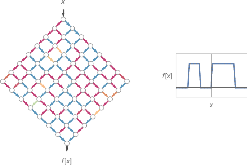
Wolfram’s “Minimal Models” post asks how much structure a neural net actually needs to learn, and answers it by stripping a standard dense network down to a sparse, geometric “mesh”: instead of every node connecting to every node in the next layer, each node connects to only two neighbors, so the whole network fans out from input to output like a diamond. That is exactly what a physical optical circuit already looks like -- Light traveling through a chip only ever interacts with its immediate neighboring channels, not with every channel at once.
In[]:=
eluNet=Import["eluNet_free_v1.wlnet"];reluNet=Import["reluNet_v1.wlnet"];phaseNet=Import["simplePhaseNet.wlnet"];phasebetaNet=Import["phaseCurvature_beta0.1_full_v2.wlnet"];
In[]:=
conv[inputSize_]:=NetGraph[{PaddingLayer[{{1,1}}],Splice@Table[NetChain[{PartLayer[{i;;i+1}],LinearLayer[1]},"Input"->{inputSize+2}],{i,inputSize+1}],CatenateLayer[]},{Splice@Table[1->1+i,{i,inputSize+1}],Splice@Table[1+i->1+inputSize+2,{i,inputSize+1}]}]createDiamondNet[steps_Integer,innerActivation_:ElementwiseLayer["ELU"],finalActivation_:ElementwiseLayer["ELU"]]:=NetChain[{FunctionLayer[{#}&],Splice@Most@Flatten@Table[{conv[i],innerActivation},{i,steps}],finalActivation,PartLayer[steps/2+1]}]SeedRandom[1234];trainingx=RandomReal[{-3,3},5000];trainingy=piecewise/@trainingx;trainingData=trainingx->trainingy;testx=Range[-3.,3.,0.01];truey=piecewise/@testx;trainMesh[act_,rounds_:2000,bs_:500]:=NetTrain[createDiamondNet[14,act,act],trainingData,All,MaxTrainingRounds->rounds,BatchSize->bs,LearningRate->0.01]testMSE[net_]:=Mean[(net[testx]-truey)^2](*Trainedtofitafixeddiscontinuouspiecewisestepfunctionon.*)
[-3, 3]
The Optics in the Mesh
The Optics in the Mesh
The general rotation, symbolic notation.
In[]:=
R[phi_]:={{Cos[phi],Sin[phi]},{-Sin[phi],Cos[phi]}};MatrixForm[R[phi]]
Out[]//MatrixForm=
Cos[phi] | Sin[phi] |
-Sin[phi] | Cos[phi] |
R is orthogonal for every phi
In[]:=
Simplify[R[phi].Transpose[R[phi]]]//MatrixFormSimplify[Det[R[phi]]]
Out[]//MatrixForm=
1 | 0 |
0 | 1 |
Out[]=
1
A real,trained node from phaseNet, not a toy example, after applying the trig functions:
In[]:=
phi11=First[Normal[NetExtract[phaseNet,{2,2,"phi","Array"}]]];numericMatrix=R[phi11];MatrixForm[numericMatrix]
Out[]//MatrixForm=
-0.930179 | -0.367108 |
0.367108 | -0.930179 |
Plugging in the trained phase φ ≈ 3.517 from an actual node in phaseNet, along with an example input pair (left, right) = (0.5, 1.2), gives a concrete numeric instance of the rotation :
In[]:=
input={0.5,1.2};output=numericMatrix.input;{"phi"->phi11,"input"->input,"output"->output,"|input|"->Norm[input],"|output|"->Norm[output]}
Out[]=
{phi3.51749,input{0.5,1.2},output{-0.905618,-0.93266},|input|1.3,|output|1.3}
Representing the phase change visually.
Representing the phase change visually.
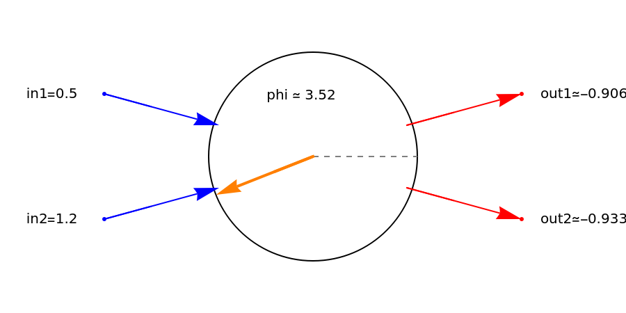
Each node in the mesh takes two incoming values (the left ports) and rotates them by a single learned angle φ, shown here as a “hand” sweeping out from the 12 o’clock reference. The outer circle marks the unit circle: because the rotation matrix R[φ] is orthogonal, the hand’s tip can slide around the circle but never leave it, which means that the node can redirect the input, but never amplify it.
The two right-hand ports show where that same energy comes out after the turn: φ ≈ 3.52 rad rotates the input pair (0.5, 1.2) into (−0.906, −0.933), same length (≈1.3), new direction.
The two right-hand ports show where that same energy comes out after the turn: φ ≈ 3.52 rad rotates the input pair (0.5, 1.2) into (−0.906, −0.933), same length (≈1.3), new direction.
Out[]=
Why ReLU Fails on a Structured Mesh?
Why ReLU Fails on a Structured Mesh?
At every layer, multiplies the correction signal by each unit's slope: if the unit's pre-activation is positive, which is the angle θ if negative. In a densely-connected network there are millions of alternate routes around a dead unit; in this mesh (2 connections per node, 14 layers deep) there are almost none, and a dead node stays dead forever because the signal that would revive it can never reach it.
1
In[]:=
deadNodesPerLayer[net_,xs_]:=Table[Count[Transpose[NetTake[net,2k][xs]],col_/;Max[col]<=0],{k,14}]deadFraction[net_,xs_]:=Total[deadNodesPerLayer[net,xs]]/119.{deadFraction[eluNet,testx],deadFraction[reluNet,testx]}
Out[]=
{0.0504202,0.882353}
ELU differs from ReLU by one detail: its off-state slope is small but never exactly zero, so the signal arrives everywhere as a whisper instead of silence.
Out[]=
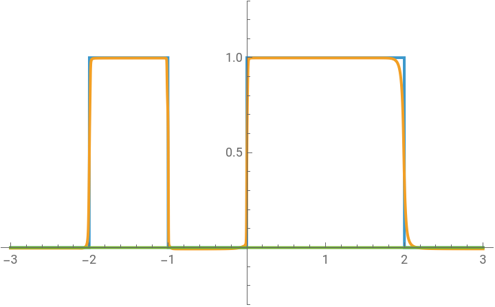


The ELU mesh tracks the step function closely; the ReLU mesh collapses to a flat line near zero.
Watching It Happen: the Training Loss Curve
Watching It Happen: the Training Loss Curve
The dead-node fraction explains why ReLU fails, but the training curve itself shows it directly. Below is a short, 100-round rerun of each net a fresh training run purely to capture the loss trajectory, not the exact same weights as the fully-trained, saved nets above, since a different random initialization won't reproduce bit-identical numbers, but the shape is the reproducible.
In[]:=
resEluQuick=trainMesh[ElementwiseLayer["ELU"],100]resReluQuick=trainMesh[ElementwiseLayer[Ramp],100]
Three distinct shapes: ReLU sits dead flat at the constant-zero baseline (≈0.51) for all 100 rounds, the gradient literally cannot reach most of the mesh, so there is nothing pulling the loss down. ELU (free weights) holds near the same baseline for its first ~15 rounds, then collapses sharply to ≈0.01 within another ~15 rounds.
Phase-constrained ELU never plateaus this hard, but descends much more slowly and gradually, consistent with needing the full 3000 rounds (not 100) to reach its eventual 0.129 — the rotation constraint costs training speed as well as final accuracy.
Conclusion: the ReLU failure here is a training problem (dying gradients), ReLU could represent the target function, it just can't learn it inside a mesh this sparse.
Phase-constrained ELU never plateaus this hard, but descends much more slowly and gradually, consistent with needing the full 3000 rounds (not 100) to reach its eventual 0.129 — the rotation constraint costs training speed as well as final accuracy.
Conclusion: the ReLU failure here is a training problem (dying gradients), ReLU could represent the target function, it just can't learn it inside a mesh this sparse.
Constraining Weights to Be Physically accurate — the Phase Mesh
Constraining Weights to Be Physically accurate — the Phase Mesh
How are we constraining
How are we constraining
Every node’s two weights already tend to land near the unit circle on their own, even with no constraint forcing them there. That’s a hint that this network doesn’t actually need full freedom to do its job, it’s already gravitating toward exactly the kind of restricted, rotation-like behavior a real optical device would be limited to.
Visualizing a triangular mesh
Visualizing a triangular mesh
Read the triangle bottom to top . The narrow point at the bottom is the raw input, and each row above it is one layer deeper into the network, ending at the wide row on top, the last layer, right before a single node' s value gets read off as the final answer . Left - to - right within a row is just that node' s position
layerOutputs runs the trained eluNet—the version with ordinary, unconstrained weights—over all 601 test points and records what every node in every one of the 14 layers actually outputs . nodeBrightness[k, j] then reduces that down to one number per node :
Building the meshes
Building the meshes
The triangle shows a network that only ever grows: 1 node → 2 → 3 → ... → 15 across the 14 layers, and the final answer is just one node picked out of that widest layer — no further combining happens after that. The diamond shows a network that grows the same way, then keeps combining pairs of nodes together on the way back down — 15 → ... → 3 → 2 → 1 . Its just different ways to represent the same thing.
Each dot is one node, placed in the network . Its color shows how "alive" it is—for every one of the 601 test inputs we record the node' s output, take the mean of its absolute value and color it on a log scale from dark/cool (near - silent across the whole input range) to bright orange or white (strong, consistent signal) . This mesh runs broadly hot, with strong activity scattered densely across nearly every layer
Phase - constrained mesh (phasebetaNet, β = 0.1) : The same exact procedure is run here, so any visual difference is a real behavioral difference, not a difference in measurement . This mesh is visibly calmer and more uniform throughout, consistent with nodes that can only rotate energy, never amplify it . There is a significant amount of dead nodes available shown which shows, this NET cannot amplify a dying signal.
Why These Graphs Don't Look Like a Normal Neural Network's
Why These Graphs Don't Look Like a Normal Neural Network's
It's worth exploring the value-propagation plots (the "fan" traces) look nothing like what you'd get from tracing hidden-unit activations in a normal, densely-connected network. Watching each of the 119 nodes' output as a function of the scalar input x, layer by layer, for both nets:
1. The first graph comes from a sparse, very regulated flow of network. In a normal dense layer, every unit mixes input from every unit in the previous layer — there's no notion of "position," so activation traces don't have obvious geometric structure. In this mesh, each node only ever combines its two immediate neighbors, and neighbors are laid out in a fixed line that mirrors the input axis. A change in x propagates outward from its own position at a fixed rate per layer, literally like a wavefront spreading through a lattice of channels.
Watching the raw matrix-multiply values propagate through all 14 layers of this net for a scan of inputs shows the effect directly — the signal fans out node by node into a broad, structured spread rather than collapsing or exploding:
Watching the raw matrix-multiply values propagate through all 14 layers of this net for a scan of inputs shows the effect directly, the signal fans out node by node into a broad, structured spread rather than collapsing or exploding, Each line is one of the 119 nodes' output as a function of input x; the symmetric bowtie spread shows the phase-constrained mesh reshaping the signal smoothly and stably across depth.
Concluding Remarks
Concluding Remarks
“is this activation good enough,” but how much deviation from linearity does a mesh actually need to learn, and what kind works?
Three findings point toward an answer. First, ReLU fails here for a structural reason, not a capability one, a sparse mesh has no alternate wiring around a dead node, so an activation with an exact-zero slope is uniquely dangerous; ELU’s slope, which is never quite zero, fixes it. Second, constraining every node to a lossless phase rotation, the real behavior of light in glass, still lets the mesh learn, just less accurately than with free weights. Third, replacing ELU with a small quadratic term (β=0.1), the same family the physical intensity law |E|² belongs to, not only trains but does better than the phase-constrained ELU baseline.
Together, these results suggest a physically realizable optical mesh doesn’t need much departure from linearity to compute, in fact a small, physically native nonlinearity can outperform a much stronger artificial one!!! Though very result here uses a node that still collapses two inputs into one output, only half of what an actual beam splitter does. Building a true two-input, two-output version is the natural next step.
Three findings point toward an answer. First, ReLU fails here for a structural reason, not a capability one, a sparse mesh has no alternate wiring around a dead node, so an activation with an exact-zero slope is uniquely dangerous; ELU’s slope, which is never quite zero, fixes it. Second, constraining every node to a lossless phase rotation, the real behavior of light in glass, still lets the mesh learn, just less accurately than with free weights. Third, replacing ELU with a small quadratic term (β=0.1), the same family the physical intensity law |E|² belongs to, not only trains but does better than the phase-constrained ELU baseline.
Together, these results suggest a physically realizable optical mesh doesn’t need much departure from linearity to compute, in fact a small, physically native nonlinearity can outperform a much stronger artificial one!!! Though very result here uses a node that still collapses two inputs into one output, only half of what an actual beam splitter does. Building a true two-input, two-output version is the natural next step.
Acknowledgments
Acknowledgments
I am grateful to my mentor Faizon Zaman, Stephen Wolfram, for the guidance throughout this project and WSRI team for this great experience.
References
References
Wolfram, S. "What's Really Going On in Machine Learning? Some Minimal Models." Stephen Wolfram Writings, August 2024. https://writings.stephenwolfram.com/2024/08/whats-really-going-on-in-machine-learning-some-minimal-models/
AI Disclosure
AI Disclosure
The following generative AI tools were used in this project: Claude. They were used for brainstorming, literature review, debugging code. All code and written content was reviewed, understood and approved by the author.
CITE THIS NOTEBOOK
CITE THIS NOTEBOOK
Learning with Light: Can a Neural Network Built Like an Optical Circuit Actually Learn?
by Keshav Seetharaman
Wolfram Community, STAFF PICKS, July 16, 2026
https://community.wolfram.com/groups/-/m/t/3761884
by Keshav Seetharaman
Wolfram Community, STAFF PICKS, July 16, 2026
https://community.wolfram.com/groups/-/m/t/3761884