Synthetic Aperture Radar (SAR) automatic target recognition (ATR) is an important capability in remote sensing. However, SAR images’ distinctive speckle noise and low resolution characteristics make it hard to distinguish. Thus, it is a fair question whether general classification models trained on everyday photos are the right tool for SAR images.
This work investigates whether a a SAR-oriented model proposed by Amrani et al., which connects a SAR-Oriented Network (SARON), Multi-Canonical Correlation Analysis (MCCA) feature fusion, and finally a linear Support Vector Machine (L2-SVM) classifier, provides a meaningful classification performance gain over other three well-known models- YOLOv8-cls, VGG-19, and ResNet-50.
SARON is freshly trained upon ATRNet-STAR, one of the newest public SAR images dataset, while other models are fine-tuned on ATRNet-STAR.
The SAR-specific network wins. SARON without feature fusion shows 94.05% top-1 accuracy, 93.66% for SARON with the full pipeline, 86.43% for YOLOv8-cls, 83.58% for VGG-19, and 90.56% for ResNet-50.
Considering that SARON is based upon VGG-19 architecture and reaches superior performance, the design choices of SARON are suitable for SAR images. However, the paper’s feature fusion step lowers the performance. Adding MCCA and SVM drops 0.39%p of accuracy.
Background
Background
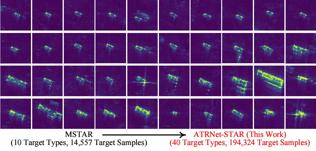
SAR images uses microwave pulses to create images, making it through clouds, smokes, and at night, which are the advantages that optical methods lack. However, the cost is that the image produes speckle, which is interference pattern that makes it low-resolution and grainy. Classification models tuned for optimal images therefore cannot be assumed to work as well under these conditions. (image from https://github.com/waterdisappear/ATRNet-STAR) There are two points that motivate the study:
◼
Modern models are mostly pre-trained on optical datasets. Will their architecture and learned features be useful for SAR images, or is SAR-specific design required?
◼
Most SAR-related deep learning studies use MSTAR, a 10-class dataset published in the 1990s. It is meaningful to scale the scope to the most recent SAR dataset available, the ATRNet-STAR dataset.
The study investigates by comparing two models on ATRNet-STAR dataset. Specifically, the main data file used for training and evaluation will be SOC_40 (ground range), which contains vehicle images of 40-class, with training and test sets having similar imaging conditions. The images description is as follows:
Dataset is available at: https://huggingface.co/datasets/waterdisappear/ATRNet-STAR
Set | #types | scene | DepressionAngle | Azimuth | Band | Polarization | #img |
train | 40 | all | 15,30,45,60 | 0~360 | X/Ku | quad | 68,091 |
test | 40 | all | 15,30,45,60 | 0~360 | X/Ku | quad | 29,169 |
Data Preparation
Data Preparation
Data Loading and Preprocessing
Data Loading and Preprocessing
Setup paths
Setup paths
In[]:=
baseDir=NotebookDirectory[];dataDir=FileNameJoin[{baseDir,"data","Amplitutde","SOC_40classes"}];trainDir=FileNameJoin[{dataDir,"train"}];testDir=FileNameJoin[{dataDir,"test"}];
Load Data
Load Data
Load training data and test data from the local folder. Then, convert class labels to integers.
Store every class name into a classList variable.
In[]:=
classList=Sort[FileNameTake[#,-1]&/@Select[FileNames["*",trainDir],DirectoryQ]];
Load training data and test data.
trainData = Flatten[Table[File[f]->label,{label, classList},{f, FileNames["*.tif", FileNameJoin[{trainDir, label}]]} ], 1];testData = Flatten[Table[File[f]->label,{label, classList},{f, FileNames["*.tif", FileNameJoin[{testDir, label}]]} ], 1];
Conversion of String labels to integers.
In[]:=
classToIndex=AssociationThread[classList->Range[Length[classList]]]; (* "2S1"1,"BMP2"2,"BRDM_2"3,"BTR_60"4,"BTR70"5, ... *)trainDataIdx=(First[#]->classToIndex[Last[#]])&/@trainData; testDataIdx=(First[#]->classToIndex[Last[#]])&/@testData;
Shuffle the data.
SeedRandom[40];trainDataIdx=RandomSample[trainDataIdx];testDataIdx=RandomSample[testDataIdx];
Building the Models
Building the Models
Function that takes a net and replaces output with a class decoder.
attachDecoder[net_]:=NetReplacePart[net, "Output"->NetDecoder[{"Class", classList}]];
YOLOv8-cls
YOLOv8-cls
VGG-19
VGG-19
ResNet-50
ResNet-50
Export Models
Export Models
SARON
SARON
Build SARON network proposed by Amrani et al.
SARON is written and trained in Python environment, using PyTorch.
The code and detailed explanation is avaialble at: https://github.com/otola03/SAR-classification
SARON is a 19-layer CNN (16 convolutional + 3 fulley-connected ), which structurally resembles VGG-19.
SARON is written and trained in Python environment, using PyTorch.
The code and detailed explanation is avaialble at: https://github.com/otola03/SAR-classification
SARON is a 19-layer CNN (16 convolutional + 3 fulley-connected ), which structurally resembles VGG-19.
◼
3x3 filters, stride 1 used: According to Amrani et al., small kernels are resilient against SAR’s noises.
◼
No Local Response Normalization, No Batch Normalization, and ReLU on every hidden layer.
◼
Unlike Amrani and his colleagues’ work, I added BatchNorm after every convolutional layer, which prevented the net not training at all.
Comparison
Comparison
Load models. The full SARON pipeline that combines SARON (CNN), MCCA, and L2-SVM was unavailable to be imported via ONNX format. Thus, the classification results on test data was reported in csv format.
yoloNet=Import[FileNameJoin[{baseDir,"models2","yolo40_final.wlnet"}]];vggNet=Import[FileNameJoin[{baseDir,"models2","vgg40_final.wlnet"}]];resnetNet=Import[FileNameJoin[{baseDir,"models2","resnet40_final.wlnet"}]];saron=Import[FileNameJoin[{baseDir, "results", "saron_soc40_wl.onnx"}], "Net"];saronEnc=NetEncoder[{"Image", {128,128},ColorSpace->"Grayscale","MeanImage"->0.5,"VarianceImage"->0.25}];saronNet=NetReplacePart[saron, "image"->saronEnc];saronPredsCSV=Import[FileNameJoin[{baseDir, "results", "saron_preds.csv"}], "CSV"];rows=Rest[saronPredsCSV]; (* file path | true label | saronCNN | saronFused (full pipeline) *)extractName[path_]:= Last[StringSplit[path, {"\\", "/"}]]; (* function to extract file name from path *)csvKeys=extractName/@rows[[All, 1]];trueLabel=AssociationThread[csvKeys->rows[[All, 2]]];cnnPred=AssociationThread[csvKeys->rows[[All, 3]]]; fusedPred=AssociationThread[csvKeys->rows[[All, 4]]];
Performance Comparison
Performance Comparison
Make predictions on test data.
testFiles=Keys[testData];testTrueLabel=Values[testData];predYolo=yoloNet[testFiles];predVgg=vggNet[testFiles];predResnet=resnetNet[testFiles];(* class list in the same index as the python environment, where SARON was built*)pyClassList=SortByFileNameTake[#,-1]&/@Select[FileNames["*",testDir],DirectoryQ], PadRight[ToCharacterCode[#],64]&; saronMargins=saronNet[testFiles];predSaron=pyClassList[[First@Ordering[#, -1]]]&/@ saronMargins;
Load predictions of fused SARON.
Comparison Table
Comparison Table
SARON, without MCCA and SVM leads the performance with the accuracy of 95.8%, followed by 90.56% of ResNet-50, 86.43% of YOLOv8-cls, and 83.58% of VGG-19. The gap between SARON and the best baseline, ResNet-50, is approximately 5.24%p.
This shows that SARON excels at classifying SAR images.
One noticeable point is that MCCA and SVM drops the performance by a small margin, which is different from what Amrani et al. claimed.
The other informative comparison is that while SARON and VGG-19 has almost identical number of parameters (~139M), they differ by almost 12%p. This difference might be explained by the use of batch normalization in SARON, VGG-19 upscaling 128x128 to 256x256, and VGG-19 being fine-tuned.
ResNet-50, although having the fewest number of parameter (~25M), outperformed the other two baseline models.
These observations show that gaps may largely be due to the design choices and architecture, rather than model size, although this work cannot clearly point out what matters the most.
Accuracy Plots
Accuracy Plots
F1-score Heatmap
F1-score Heatmap
The rows are sorted from lowest mean f1 score.
One surprising finding is that the models performed well on relatively big vehicles. The easiest vehicles are trucks and buses: SHACMAN DeLong X3000 and M3000, Yutong ZK6120HY1, Dongfeng Tianjin KR230, FAW J6P, CNHTC HOWO. The hardest are sedans and SUVs: Chery Arrizo 5, Jeep Patriot, Buick Excelle GT.
This is a predictable result, as larger vehicles tend to take up more resolution and produce richer information, while smaller sedans are less distinguishable.
SARON and SARON (MCCA + SVM) both excelled, with approximately 0.9 for every class.
F1-score of Top-10 Hardest Classes vs. The Number of Test Data
F1-score of Top-10 Hardest Classes vs. The Number of Test Data
The best score of ResNet-50 (87.2%) is still lower than SARON (CNN) and SARON (MCCA + SVM)’s lowest scores (90.7% and 88.8%). There is no class here where the baseline model performs as well as SARON models.
If the hardest classes are the fewest in the test data, that indicates the difficulty is related to scarcity. However, the table indicates otherwise. Difficulty does not follow training set’s size. Rather, these vehicles are hard because they look alike in SAR.
If the hardest classes are the fewest in the test data, that indicates the difficulty is related to scarcity. However, the table indicates otherwise. Difficulty does not follow training set’s size. Rather, these vehicles are hard because they look alike in SAR.
Conclusion
Conclusion
On the ATRNet-STAR dataset, SARON models outperforms baseline models. SARON models reached above 95% accuracy, and had no weak classes by reaching 0.9+ F1-score on all 40 classes. However, its MCCA fusion step lowered accuracy by 0.28%p, and it might be because two feature layers (fc6 and fc7) have almost identical information, making the process redundant and costly instead. VGG-19, with similar number of parameters to SARONs, performed the worst among all five models. This shows that the size of a network does not matter, but how it is designed determines the performance- which is why SARON earned the best scores.
References
References
◼
Liu, Y., Li, W., Liu, L., Zhou, J., Peng, B., Song, Y., Xiong, X., Yang, W., Liu, T., Liu, Z., & Li, X. (2026). ATRNEt-STAR: a large dataset and benchmark towards remote sensing object recognition in the wild. IEEE Transactions on Pattern Analysis and Machine Intelligence, PP, 1–18. https://doi.org/10.1109/tpami.2026.3658649
◼
Amrani, M., Bey, A., & Amamra, A. (2021). New SAR target recognition based on YOLO and very deep multi-canonical correlation analysis. International Journal of Remote Sensing, 43(15–16), 5800–5819.
https://doi.org/10.1080/01431161.2021.1953719
https://doi.org/10.1080/01431161.2021.1953719
◼
Tang, Y. (2013). Deep Learning using Linear Support Vector Machines. arXiv (Cornell University).
https://doi.org/10.48550/arxiv.1306.0239
https://doi.org/10.48550/arxiv.1306.0239
◼
This work was assisted by AI tools.
CITE THIS NOTEBOOK
CITE THIS NOTEBOOK
SARON: synthetic aperture radar oriented network
by Wonjoon Koh
Wolfram Community, STAFF PICKS, August 22, 2026
https://community.wolfram.com/groups/-/m/t/3785847
by Wonjoon Koh
Wolfram Community, STAFF PICKS, August 22, 2026
https://community.wolfram.com/groups/-/m/t/3785847