ABSTRACT (original book): “Artificial Neural Network and Deep Learning: Fundamentals and Theory” offers a comprehensive exploration of the foundational principles and advanced methodologies in neural networks and deep learning. This book begins with essential concepts in descriptive statistics and probability theory, laying a solid groundwork for understanding data and probability distributions. As the reader progresses, they are introduced to matrix calculus and gradient optimization, crucial for training and fine-tuning neural networks. The book delves into multilayer feed-forward neural networks, explaining their architecture, training processes, and the backpropagation algorithm. Key challenges in neural network optimization, such as activation function saturation, vanishing and exploding gradients, and weight initialization, are thoroughly discussed. The text covers various learning rate schedules and adaptive algorithms, providing strategies to optimize the training process. Techniques for generalization and hyperparameter tuning, including Bayesian optimization and Gaussian processes, are also presented to enhance model performance and prevent overfitting. Advanced activation functions are explored in detail, categorized into sigmoid-based, ReLUbased, ELU-based, miscellaneous, non-standard, and combined types. Each activation function is examined for its properties and applications, offering readers a deep understanding of their impact on neural network behavior. The final chapter introduces complex-valued neural networks, discussing complex numbers, functions, and visualizations, as well as complex calculus and backpropagation algorithms. This chapter provides a comprehensive overview of complex activation functions and their unique properties. This book equips readers with the knowledge and skills necessary to design, and optimize advanced neural network models, contributing to the ongoing advancements in artificial intelligence. CITATION (original full book): M. M. Hammad (2024), Artificial Neural Network and Deep Learning: Fundamentals and Theory, arXiv:2408.16002. https://doi.org/10.48550/arXiv.2408.16002
Bridging Theory and Practice: The Dual Approach of This Book
Bridging Theory and Practice: The Dual Approach of This Book
Many books on neural networks and deep learning tend to lean either heavily on theoretical aspects, with dense mathematical formulations, or focus predominantly on computational algorithms, often at the expense of a solid mathematical foundation. This book adopts a balanced approach that bridges the gap between these extremes. By seamlessly integrating theoretical principles with practical implementation, it empowers learners to fully harness the power of neural networks and deep learning in their pursuit of excellence across various domains.
However, attempting to cover both the theoretical concepts and computational algorithms exhaustively within a single volume would be impractical. To ensure a thorough exploration of both aspects, this book is divided into two complementary parts. The first part is titled “Artificial Neural Network and Deep Learning: Fundamentals and Theory.” The second part is titled “Neural Network and Deep Learning with Mathematica.” For each theoretical chapter in the first part, there is a corresponding chapter in the second part. We strongly recommend that after completing each theoretical chapter, you explore the corresponding practical implementation chapter in the complementary volume. This dual approach will provide you with a well-rounded understanding and the skills necessary to excel in this field.
The book “Neural Network and Deep Learning with Mathematica” adopts a refreshingly code-centric approach, enabling you to solidify your understanding through hands-on practice. Nearly all the concepts introduced are accompanied by illustrative code examples, making the learning experience both practical and tangible. Even the figures in the first part are generated using these code examples, emphasizing the code-first methodology. To ensure accessibility and ease of understanding, the code examples are deliberately crafted in a simple format, prioritizing readability over efficiency and generality. In line with our instructional philosophy, each code example serves a dual purpose: not only does it demonstrate a specific deep learning concept, but it also simultaneously introduces and reinforces Mathematica programming techniques. Readers will learn how to leverage Mathematica to perform complex neural network and deep learning calculations, simulate data, and create visual representations of their findings.
Chapter 7: Strategies for generalization and hyper-parameter tuning
Chapter 7: Strategies for generalization and hyper-parameter tuning
In this chapter, we delve into some of the most critical concepts and methodologies that form the backbone of machine learning, guiding the development of models that are not only powerful but also robust and generalizable across various scenarios. We focus on the aspects of Neural Network (NN) training that determine how effectively a model can generalize from training data to unseen data. Generalization is the ultimate test of a NN’s performance, assessing its ability to apply learned patterns to new datasets.
The following are sample illustrative code examples corresponding to the first two parts of this chapter.
7.1 Overfit
7.1 Overfit
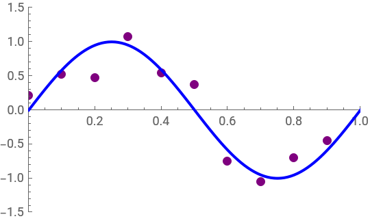
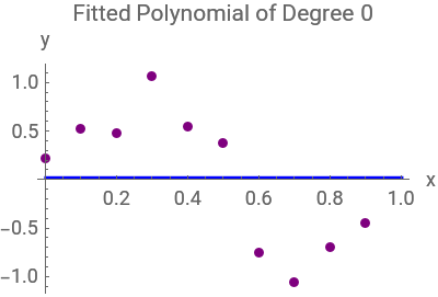
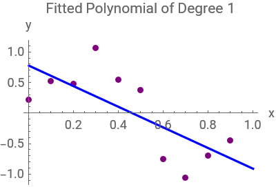
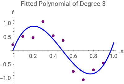
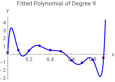
The code aims to analyze the performance of polynomial regression models in approximating a sinusoidal function with added noise. It generates a set of training data points by sampling from the sinusoidal function with random noise. Subsequently,polynomials of different degrees (0,1,3,and 9) are fitted to the training data to capture the underlying relationship between the input variable (x) and the target variable (y). The code then visualizes the training data along with the original sinusoidal function curve to understand the data distribution. Additionally,separate plots are generated for each fitted polynomial curve to assess their performance in approximating the underlying function. Through this analysis,the code aims to evaluate the trade-off between model complexity and goodness of fit,providing insights into the effectiveness of polynomial regression models for the given dataset:
Generate random seed for reproducibility :
SeedRandom[134];
Generate training data : sinusoidal function with added random noise
trainingData=Table[{x,Sin[2πx]+RandomVariate[NormalDistribution[0,0.3]]},{x,0,0.9,0.1}];
Fit polynomials of different degrees to the training data :
fittedPolynomials=Table[Fit[trainingData,Table[x^i,{i,0,m}],x],{m,{0,1,3,9}}]
Plot the training data with the original sinusoidal function curve :
ListPlot[trainingData,PlotStyle->{PointSize[0.025],Purple},PlotRange->{{0,1},{-1.5,1.5}},FrameLabel->{"x","y"},AxesOrigin->{0,0},ImageSize->270,Epilog->{Blue,Thick,Line[Transpose[{Range[0,1,0.01],Sin[2πRange[0,1,0.01]]}]]}](*Ploteachfittedpolynomialseparately:*)Table[Show[ListPlot[trainingData,PlotStyle->{PointSize[0.025],Purple},PlotRange->All,ImageSize->200],Plot[fittedPolynomials[[i]],{x,0,1},PlotStyle->Blue],PlotRange->All,AxesLabel->{"x","y"},PlotLabel->"Fitted Polynomial of Degree "<>ToString[{0,1,3,9}[[i]]]],{i,Length[fittedPolynomials]}]
Out[]=
{0.0209197,0.780035-1.68692x,0.0221099+9.33508x-28.6867+19.6234,0.213963+236.151x-5876.84+57575.-294786.+877743.-1.57544×+1.67889×-977501.+239311.}
2
x
3
x
2
x
3
x
4
x
5
x
6
10
6
x
6
10
7
x
8
x
9
x
Out[]=
Out[]=
,
,
,
The code aims to assess the performance of polynomial regression models by evaluating the root mean square (RMS) errors for varying polynomial degrees using both training and test datasets. It begins by generating a synthetic dataset composed of sinusoidal data points with added random noise. Subsequently,it defines a function to compute the residual sum of squares (RSS) to quantify the discrepancy between the fitted polynomial curves and the actual data. After generating a finer-resolution test dataset, the code fits polynomial models of increasing degrees to the training data and calculates the RMS errors for both training and test datasets. The resulting RMS error values are plotted against the polynomial degrees, providing insights into the trade-off between model complexity and generalization performance,aiding in the selection of an optimal model complexity to avoid underfitting or overfitting:
SeedRandom[12];
Generate training dataset with sinusoidal function and noise:
trainingData=Table[{x,Sin[2πx]+RandomVariate[NormalDistribution[0,0.3]]},{x,0,1,0.1}];
Define a function to calculate Root Mean Square Error (RSS) :
calculateRSS[data_,fit_]:=Sqrt[(1/Length[data])*Total[(fit-data[[All,2]])^2]];
Generate test dataset with finer resolution :
testData=Table[{x,Sin[2πx]+RandomVariate[NormalDistribution[0,0.2]]},{x,0,1,0.01}];
Define polynomial orders to test :
orders=Range[0,10];
Calculate RMS for training data for each polynomial order:
trainingRMS=Table[(*Fitapolynomialofdegreemtothetrainingdata:*)fit=Fit[trainingData,Table[x^i,{i,0,m}],x];(*Generatefittedvaluesforeachtrainingdatapoint:*)fitValues=Table[fit,{x,trainingData[[All,1]]}];(*CalculateRSSbetweenfittedvaluesandactualtrainingdata:*)calculateRSS[trainingData,fitValues],{m,orders}];
Calculate RMS for test data for each polynomial order :
testRMS=Table[(*Fitapolynomialofdegreemtothetrainingdata:*)fit=Fit[trainingData,Table[x^i,{i,0,m}],x];(*Generatefittedvaluesforeachtestdatapoint:*)fitValues=Table[fit,{x,testData[[All,1]]}];(*CalculateRSSbetweenfittedvaluesandactualtestdata:*)calculateRSS[testData,fitValues],{m,orders}];
Plot the results:
ListLinePlot[(*PlotbothtrainingandtestRMSerrors:*){Transpose[{orders,trainingRMS}],Transpose[{orders,testRMS}]},PlotLegends->{"Training RMS Error","Test RMS Error"},AxesLabel->{"M","RMS"},PlotRange->All,ImageSize->250]
The goal of this code is to illustrate how the behavior of fitted polynomial curves changes as the size of the dataset varies. By generating datasets of different sizes and fitting polynomial curves of the same degree to each dataset, the code aims to demonstrate the relationship between dataset size and model complexity. Specifically, it seeks to show that as the dataset size increases,the overfitting problem becomes less severe, allowing for the fitting of more complex models without encountering significant overfitting. The code generates synthetic data points simulating a sinusoidal function with added random noise,creating two datasets with different step sizes. It then fits polynomial curves of degree 9 to each dataset and visualizes the data points alongside the corresponding fitted curves:
Seed the random number generator for reproducibility:
Function to generate data points:
Function to fit a polynomial to the data :
Use built - in function Fit to fit a polynomial of given degree :
Use built - in function Fit to fit a polynomial of given degree :
Function to plot the data along with the fitted curve:
The code aims to analyze the performance of polynomial regression models in approximating a sinusoidal function with added noise. It begins by generating multiple training datasets with varying levels of noise, using a sinusoidal function as the underlying pattern. Then, it fits polynomials of different degrees to each dataset,allowing for exploration of the relationship between model complexity and goodness of fit. The fitted polynomials are visualized alongside the original training data,aiding in the assessment of how well the models capture the underlying sinusoidal function. Through this analysis,the code aims to provide insights into the effectiveness of polynomial regression models in capturing complex relationships while navigating the trade-off between model complexity and accuracy:
Define a function to generate training data with specified noise level :
The code generates synthetic noisy data representing a mathematical function and trains a multilayer perceptron (MLP) neural network on this data. The MLP architecture comprises two hidden layers with 150 units each, utilizing hyperbolic tangent activation functions. Following training,the network's performance is evaluated on a separate test dataset to assess its generalization capabilities. Despite achieving low loss on the training data,the trained model demonstrates poor performance on the test set,indicating potential overfitting. This disparity is visually demonstrated by comparing the model's predictions to both the training and test data,highlighting the need for careful evaluation of model generalization beyond training performance:
Generate synthetic noisy training data based on a Gaussian function and add Gaussian noise :
Visualize the training data and the noise - free original function for comparison:
7.2 Performance Measurements
7.2 Performance Measurements
The code is designed to create synthetic data from a Gaussian distribution, construct a neural network with two hidden layers,and train this network using the generated data with added noise. The main objectives are to accurately model the underlying data patterns,optimize the network parameters for best performance, and ensure the model's generalization to new, unseen data through rigorous training and validation. The training process,limited to 50 rounds, includes monitoring metrics such as mean deviation, mean square error, R-squared, and standard deviation to assess accuracy and prevent overfitting,providing a comprehensive approach to training and evaluating the neural network's performance. All the results from the training session are stored in the NetTrainResultsObject. This object provides a convenient way to access various details about the training process, including performance metrics, the best model configuration, and other properties that can help in analyzing and understanding the behavior and effectiveness of the trained neural network. You can query this object for specific details like validation losses, training metrics, and the final trained model, which are crucial for further evaluation and refinement of your model:
Define the underlying data function as a Gaussian distribution:
Set the noise level for generating synthetic data:
Generate training data : sample points from the defined function and add Gaussian noise:
Generate validation data in the same manner but with fewer points:
Define a neural network with two hidden layers and one output layer:
Obtain a NetTrainResultsObject for a training session:
Access various details about the training process from NetTrainResultsObject :
Similar to the previous code, this version accesses various details about the training process by utilizing'ValidationMeasurements':
This code explicitly specifies "ValidationMeasurements" as a property to retrieve in the NetTrain function. This shows a clear intent to focus on and directly access detailed validation metrics throughout the training process. This approach ensures that these specific metrics are highlighted and analyzed,which is particularly useful for a more detailed performance evaluation. Note that, the previous code does not explicitly specify a focus on validation measurements within the NetTrain function. It saves all training results in a NetTrainResultsObject,which can store a wide range of information but does not emphasize specific validation metrics unless manually accessed later:
This code explicitly specifies "ValidationMeasurements" as a property to retrieve in the NetTrain function. This shows a clear intent to focus on and directly access detailed validation metrics throughout the training process. This approach ensures that these specific metrics are highlighted and analyzed,which is particularly useful for a more detailed performance evaluation. Note that, the previous code does not explicitly specify a focus on validation measurements within the NetTrain function. It saves all training results in a NetTrainResultsObject,which can store a wide range of information but does not emphasize specific validation metrics unless manually accessed later:
Define the underlying data function as a Gaussian distribution:
Set the noise level for generating synthetic data:
Generate training data : sample points from the defined function and add Gaussian noise:
Generate validation data in the same manner but with fewer points:
Define a simple neural network structure:
Associations of the final value of all measurements can be obtained after training by specifying “ValidationMeasurements” as properties in NetTrain[net, data, properties]:
Access various details about the training process from NetTrainResultsObject:
The code aims to generate a synthetic dataset within a unit disk, label the data based on proximity to the center,and visualize this distribution. It constructs a simple neural network for binary classification,which includes linear and non-linear layers to capture complex patterns. The network is trained using the generated data, validated with a separate set,and evaluated using several performance metrics. The training process is visualized through a contour plot showing the decision boundaries and other training-related plots like the confusion matrix. The goal is to demonstrate the complete workflow of data preparation, model training,and performance evaluation in a neural network application:
Generate 1000 random points within a unit disk for training :
Assign labels based on whether the point’ s distance from the origin is less than 0.5 :
Combine the points and labels into training data :
Generate 500 random points within a unit disk for validation :
Assign labels using the same criteria as for the training set :
Combine the points and labels into validation data
Visualize the synthetic training set with different colors for each class :
Similar to the previous code, this version accesses various details about the training process by utilizing ‘ ValidationMeasurements’ :
The introduction of “ValidationMeasurements” in NetTrain suggests a focus on in-depth analysis and monitoring of the model’s performance specifically on the validation data throughout the training process. This can be critical for understanding how well the model generalizes to new, unseen data and for making adjustments to model parameters or training procedures based on validation feedback:
The introduction of “ValidationMeasurements” in NetTrain suggests a focus on in-depth analysis and monitoring of the model’s performance specifically on the validation data throughout the training process. This can be critical for understanding how well the model generalizes to new, unseen data and for making adjustments to model parameters or training procedures based on validation feedback:
Generate 1000 random points within a unit disk for training :
Assign labels based on whether the point’ s distance from the origin is less than 0.5 :
Combine the points and labels into training data :
Generate 500 random points within a unit disk for validation :
Assign labels using the same criteria as for the training set :
Combine the points and labels into validation data :
Define a neural network with two linear layers and activation functions :
CITE THIS NOTEBOOK
CITE THIS NOTEBOOK
Artificial neural network and deep learning: fundamentals and theory
by Mohamed Hammad
Wolfram Community, STAFF PICKS, September 4, 2024
https://community.wolfram.com/groups/-/m/t/3266534
by Mohamed Hammad
Wolfram Community, STAFF PICKS, September 4, 2024
https://community.wolfram.com/groups/-/m/t/3266534