ORIGINAL ARTICLE: Aditya Prakash, Abhishek Kumar, Colin Benjamin, Impurity reveals distinct operational phases in quantum thermodynamic cycles, Phys.Rev.E 106, 054112 (2022). DOI: https://doi.org/10.1103/PhysRevE.106.054112
Article Abstract: We analyze the effect of impurity on the work output and efficiency of quantum Otto and quantum Carnot heat cycles, modeled as a single quantum particle in an infinite square well potential, which is the working substance. We solve this quantum mechanical system perturbatively up to first and second order in strength of the impurity for strong - and weak - coupling regimes, respectively. We derive the analytical expressions of work and efficiency for the strong - coupling regime to the first order in the strength parameter. The threshold value of the strength parameter in weak coupling is obtained up to which the numerical result agrees with the perturbative result for a repulsive and attractive impurity. To our surprise, an embedded impurity unlocks new operational phases in the system, such as a quantum heat engine, quantum refrigerator, and quantum cold pump. In addition, the efficiency of the quantum Otto heat engine is seen to reach Carnot efficiency for some parameter regimes. The cooling power and coefficient of performance of the quantum refrigerator and quantum cold pump are nontrivially affected by the impurity.
Introduction
Introduction
Our paper delves into the quantum Otto and Carnot heat cycles. In the realm of quantum thermodynamics, while others have explored work outputs and efficiencies for various quantum cycles, the impact of impurities has remained unexplored. We've introduced an impurity, used quantum thermodynamic principles, and uncovered intriguing effects. What sets our work apart is the revelation of diverse operational phases by adjusting system parameters: heat engine, cold pump, refrigerator – all achievable. Our work opens doors to a versatile device, enabling seamless shifts between operational modes. Furthermore, it aligns with current research trends, as unconventional thermodynamic properties of low - dimensional systems garner significant attention.
Work and heat calculation
Work and heat calculation
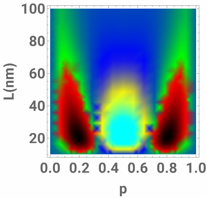
This code depicts the case when strength of the impurity is varied stroke-wise. This code can be used to reproduce Fig. 8 in the paper.Work will be computed using the following expression:To calculate this we use the “Sum” function offered by Wolfram Mathematica.

Identifying distinct thermodynamic phases
Identifying distinct thermodynamic phases
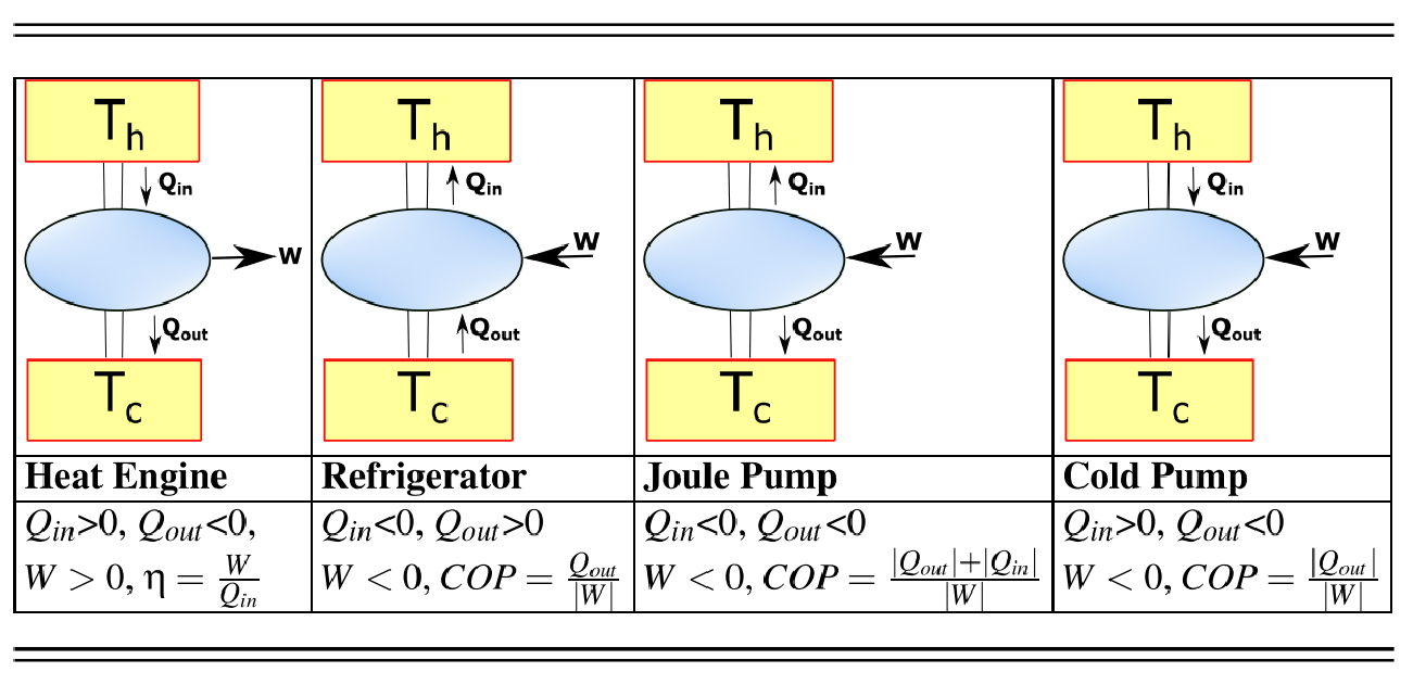
Distinct thermodynamic phases can be identified by comparing the relative signs of work done and heat absorbed/emitted as shown in the table below (Table I in the paper):
Initializing functions
Initializing functions
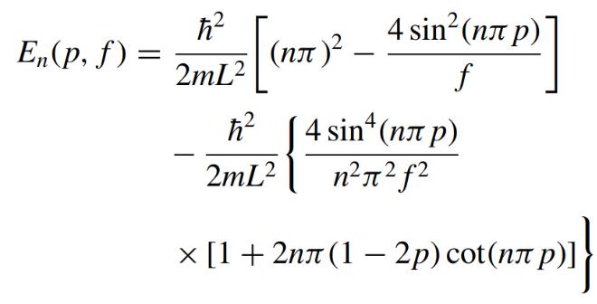
1) ENE: Returns the eigenvalue of the system in weak coupling regime (Eq.15 in the paper) as shown below:2) ZA: Returns the partition function of our system, which is given by:

Code:
Code:
This in electron volt; 0.0423 is the value of h^2/2 mL^2 in meV, i.e., in milli electron volt where h cut is taken in electron volt and m is mass of e. L = 30 nm.
ENE[n6_,g6_,p6_,L6_]:=38.19/(L6^2)*((n6*Pi)^2-(4/g6)*((Sin[n6*Pi*p6])^2)-(4/(g6*n6*Pi)^2)*((Sin[n6*Pi*p6])^4+(2*Pi*n6)*(1-2*p6)*((Sin[n6*Pi*p6])^3)*Cos[n6*Pi*p6]));
Now lets define partition function for perturbative energy:
ZA[p6_,st6_,T6_,L6_]:=Sum[Exp[-(38.19/((L6^2)T6))*((n6*Pi)^2-(4/st6)*((Sin[n6*Pi*p6])^2)-(4/(st6*n6*Pi)^2)*((Sin[n6*Pi*p6])^4+(2*Pi*n6)*(1-2*p6)*((Sin[n6*Pi*p6])^3)*Cos[n6*Pi*p6]))],{n6,1,100}]
Note that whenever T is written, then the Boltzmann Constant is also included in it. Defining Temperature, in all these values Boltzmann constant is included. If your temperature is x then put x*0.086173333.
Initialize Variables:
Initialize Variables:
atc6=0.12926;(*KmultipliedbyColdreservoirtemperaturehereitis1.5K*)ath6=0.43086665;(*Hotreservoir1temp*5K*)ath7=1.02546263;(*Hotreservoir2temp*11.9K*)ath8=2.1543333;(*Hotreservoir3temp*K25*)asth=1;(*Strengthathotreservoir*)astc=-1;(*strengthincoldreservoir*)k=0.08617;(*ValueofboltzmanconstantinmeV*)
Computing Work done while varying position and length of the system cycle-wise and strength is varied stroke-wise:
colors={Black,Red,Green,Blue,Cyan,Yellow};w=List@@@ColorConvert[colors,"RGB"].{0.3,0.3370,0.5}colorfn=Evaluate[Blend[{w,colors},#]]&;
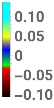
DensityPlot[((Sum[ENE[n6,asth,p6,L]/(Exp[ENE[n6,asth,p6,L]/ath8]),{n6,1,100}]/ZA[p6,asth,ath8,L])-(Sum[ENE[n6,asth,p6,L]/(Exp[(ENE[n6,astc,p6,L])/atc6]),{n6,1,100}]/ZA[p6,astc,atc6,L])-(Sum[ENE[n6,astc,p6,L]/(Exp[(ENE[n6,asth,p6,L])/ath8]),{n6,1,100}]/ZA[p6,asth,ath8,L])+(Sum[ENE[n6,astc,p6,L]/(Exp[(ENE[n6,astc,p6,L])/atc6]),{n6,1,100}]/ZA[p6,astc,atc6,L])),{p6,0,1},{L,10,100},PlotRangeAll,PlotTheme"Scientific",FrameLabel{"p","L(nm)"},LabelStyle{FontSize25,Directive[Bold]},PlotLegendsBarLegend[Automatic,LegendMarkerSize180,LegendFunction"Frame",LegendMargins5,LegendLabel"W(meV)"],ColorFunctioncolorfn]
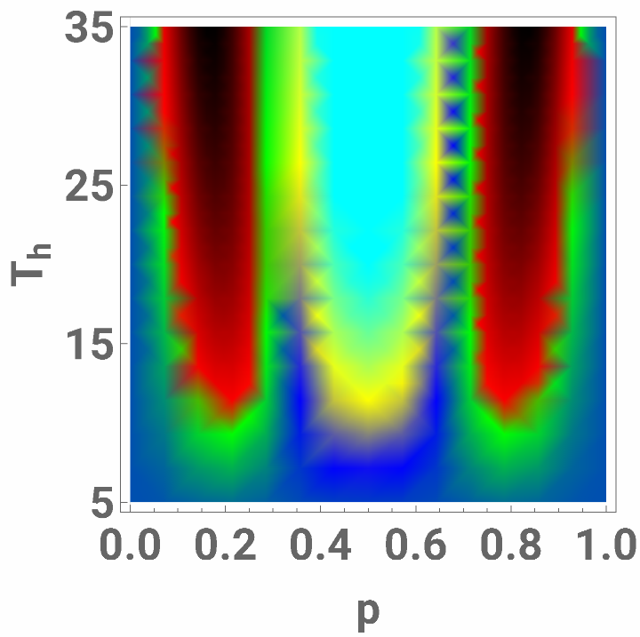
Varying p (position) and Th (hot reservoir temperature) with L = 25nm
Varying p (position) and Th (hot reservoir temperature) with L = 25nm
L=25;
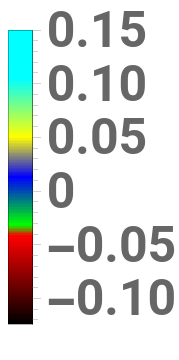
DensityPlot[((Sum[ENE[n6,asth,p6,L]/(Exp[ENE[n6,asth,p6,L]/(k*T)]),{n6,1,100}]/ZA[p6,asth,(k*T),L])-(Sum[ENE[n6,asth,p6,L]/(Exp[(ENE[n6,astc,p6,L])/atc6]),{n6,1,100}]/ZA[p6,astc,atc6,L])-(Sum[ENE[n6,astc,p6,L]/(Exp[(ENE[n6,asth,p6,L])/(k*T)]),{n6,1,100}]/ZA[p6,asth,(k*T),L])+(Sum[ENE[n6,astc,p6,L]/(Exp[(ENE[n6,astc,p6,L])/atc6]),{n6,1,100}]/ZA[p6,astc,atc6,L])),{p6,0,1},{T,5,35},PlotRangeAll,PlotTheme"Scientific",FrameLabel{"p",Subscript["T","h"]},LabelStyle{FontSize25,Directive[Bold]},FrameTicks{{{5,15,25,35},None},{Automatic,None}},PlotLegendsBarLegend[Automatic,LegendMarkerSize180,LegendFunction"Frame",LegendMargins5,LegendLabel"W(meV)"],ColorFunctioncolorfn]
Varying f (strength) and T_h (from 1 to 50K)
Varying f (strength) and T_h (from 1 to 50K)
ph=0.5;
colors={Blue,Cyan,Yellow};w=List@@@ColorConvert[colors,"RGB"].{0.1,0.3570,0.3}colorfn2=Evaluate[Blend[{w,colors},#]]&;(*DensityPlot[x,{x,0,1},{y,0,2},AspectRatio0.1,ColorFunctioncolorfn2]*)
For Cold Pump, plotting work for p = 0.15
For Cold Pump, plotting work for p = 0.15
Computing efficiency while varying p and L (length of well) cycle-wise
Computing efficiency while varying p and L (length of well) cycle-wise
Computing efficiency varying T_h and p
Computing efficiency varying T_h and p
CITE THIS NOTEBOOK
CITE THIS NOTEBOOK
Impurity reveals distinct operational phases in quantum thermodynamic cycles
by Aditya Prakash, Abhishek Kumar, Colin Benjamin
Wolfram Community, STAFF PICKS, September 11, 2023
https://community.wolfram.com/groups/-/m/t/3010647
by Aditya Prakash, Abhishek Kumar, Colin Benjamin
Wolfram Community, STAFF PICKS, September 11, 2023
https://community.wolfram.com/groups/-/m/t/3010647