DirectionalDerivatives::usage="Given a vector = {,}, the directional derivative of f at the point (x, y) in the direction of is: f(x, y) = (x, y)+ (x, y) = {(x, y), (x, y)}. or in three variables: f(x, y, z) = (x, y, z)+ (x, y, z) + (x, y, z) = {(x, y, z), (x, y, z), (x, y, z) }. . This is also how the directional derivative can be defined: f = ∇f. u, where ∇f it is the gradient of f. ∇f(x, y) = {(x,y), (x,y)}, in three variables: ∇f(x, y, z) = {(x,y,z), (x,y,z), (x,y,z}}, it is valid for n variables. If ∇f ≠ 0, then ∇f give the direction of the largest increase in f, and - ∇f give the direction of the largest decrease in f. Find the directional derivative of the function f[x, y] = Cos[x y] at the point , π in the direction = {Cos[θ], Sin[θ]}. Graph the function in the interval of 0 ≤ θ ≤ 2π, and find the value where the extreme occurs. So for these values of θ, verify that corresponds to ∇f or - ∇f. References: Hollis, Selwyn. CalcLabs with Mathematica. Multivariable Calculus. Cengage: p.98 4a. Ed, 2010; Personal. ";
u
u
1
u
2
u
D
u
f
x
u
1
f
y
u
2
f
x
f
y
u
D
u
f
x
u
1
f
y
u
2
f
z
u
3
f
x
f
y
f
z
u
D
u
f
x
f
y
f
x
f
y
f
z
1
4
u
u
In[]:=
f[x_,y_]:=Cos[xy];α=ResourceFunction["DirectionalD"][f[x,y],{Cos[θ],Sin[θ]},{x,y}]/.x,yπ;Print[α];
1
4
--
πCos[θ]
2
Sin[θ]
4
2
In[]:=
gradf[x_,y_]=Grad[f[x,y],{x,y}];p0=,π,0;tanvec=Appendgradf,π,,π,0//N;Withp={x,y,f[x,y]}/.x,yπ,q=gradvec,r=tanvec,ShowPlot3D[f[x,y],{x,0,2π},{y,0,2π},MeshFalse,PlotRangeAll,PlotStyleOpacity[.3],PlotRangeAll,AxesLabel->(Style[#,15,Blue]&/@{"X","Y","Z"}),BoxRatiosAutomatic,AxesOrigin{0,0,0},BoxedFalse,PlotLabelStyle[Framed["Directional derivative (black), tangent vector (red) and gradient (blue):"],16,Blue,BackgroundYellow]],Graphics3D[{Blue,Point[p0],Arrowheads[.05],Arrow[Tube[{p0,p0+q}]]}],Graphics3D[{Red,Point[p],Arrowheads[.05],Arrow[Tube[{p,p+r}]]}],Graphics3DBlack,Point[p],Arrowheads[.05],ArrowTubep,p+Cos[θ],Sin[θ],--/.θ2π
1
4
1
4
gradf,π.gradf,π
//N;gradvec=Appendgradf1
4
1
4
1
4
1
4
πCos[θ]
2
Sin[θ]
4
2
Out[]=

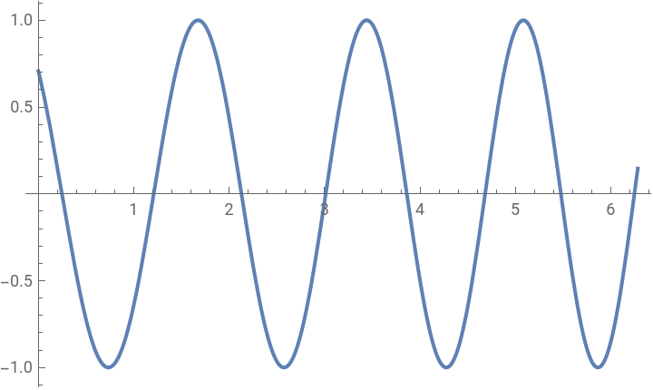
Next, the values of t for which decrease the function, where the minimums exist:
In[]:=
gradLen=N
gradf,π.gradf,π
1
4
1
4
Out[]=
2.22846
In[]:=
u=-gradf,πgradLen
1
4
Out[]=
{0.996849,0.0793267}
In[]:=
{x[t_],y[t_]}=,π+tu
1
4
Out[]=
+0.996849t,π+0.0793267t
1
4
In[]:=
f[x[t],y[t]]//SimplifyPlot[f[x[t],y[t]],{t,0,2π}]
Out[]=
Sin[0.785398-3.15152t-0.0790767]
2
t
Out[]=
In[]:=
{x[t],y[t],f[x[t],y[t]]}/.t0.74
Out[]=
{-0.487668,3.08289,0.0673181}
In[]:=
{x[t],y[t],f[x[t],y[t]]}/.t2.58
Out[]=
{-2.32187,2.93693,0.859767}
In[]:=
{x[t],y[t],f[x[t],y[t]]}/.t4.31
Out[]=
{-4.04642,2.79969,0.327031}
Correspons to - ∇f, that is in the direction of decrease.
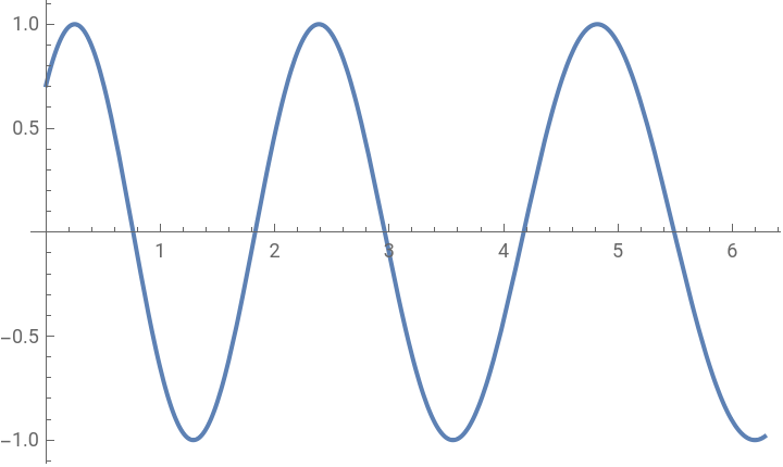
Next, the values of t for which the function increase, where the maximums exist:
u=gradf,πgradLen
1
4
{-0.9968486721503291,-0.07932669684365853}
In[]:=
{x[t_],y[t_]}=,π+tu
1
4
Out[]=
-0.996849t,π-0.0793267t
1
4
In[]:=
f[x[t],y[t]]//SimplifyPlot[f[x[t],y[t]],{t,0,2π}]
Out[]=
Sin[0.785398+3.15152t-0.0790767]
2
t
Out[]=
In[]:=
{x[t],y[t],f[x[t],y[t]]}/.t0.28
Out[]=
{-0.0291176,3.11938,0.995878}
In[]:=
{x[t],y[t],f[x[t],y[t]]}/.t2.41
Out[]=
{-2.15241,2.95042,0.997736}
Corresponds to ∇f, that is in the direction of increase.