In[]:=
numBases=100;(*Numberofbasepairs,representingasegmentofDNA*)kappa=1/10;(*Elasticityconstant,chosentoreflectthestiffness;arbitraryunit*)omegaD=2/10;(*Frequencyterm,speculativeandlowtoreflectslowdynamics*)beta=5/100;(*Nonlinearitycoefficientsmalltointroducemildnonlinearity*)
In[]:=
(*Initializealistforthex_nvariables*)variables=Table[x[n],{n,1,numBases}];(*DefinetheequationsbasedonthediscretizedversionoftheKlein-Gordonequation*)equations=Table[-kappa(x[n+1]-2x[n]+x[n-1])==omegaD^2(x[n]-betax[n]^3),{n,2,numBases-1}];
In[]:=
(*Addboundaryconditions,forexample,x[1]andx[numBases]fixedto0oranyothervalue*)boundaryConditions={x[1]==1,x[numBases]==1};
In[]:=
(*Combinetheequationswiththeboundaryconditions*)fullSystem=Join[equations,boundaryConditions];
In[]:=
(*Solvethesystemwithaninitialguessforeachvariable*)initialGuess=Table[{x[n],1/100},{n,1,numBases}];(*oranysmallvalueclosetoexpectedsolutions*)
In[]:=
solution=FindRoot[fullSystem,initialGuess,AccuracyGoal->8,PrecisionGoal->30,WorkingPrecision->50];
In[]:=
(*Extractthesolutionforplottingoranalysis*)solvedValues=Table[x[n]/.solution,{n,1,numBases}];
In[]:=
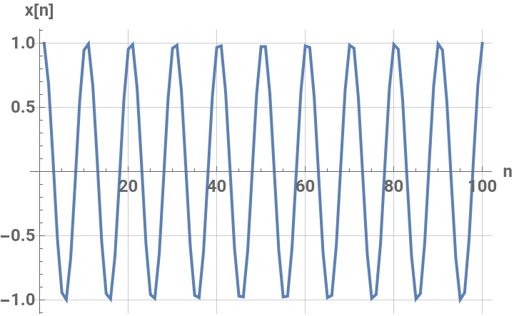
(*Optionally,youcanplotthesolutiontovisualizethestationarystates*)ListPlot[solvedValues,PlotStyle->PointSize[Medium],Joined->True,GridLines->Automatic,PlotRange->All,AxesLabel->{"n","x[n]"},LabelStyle->{"Medium",Bold}]
Out[]=