This educational example explores population growth through a progression from a basic rainbowfish population in an aquarium to a refined model utilizing differential equations. Beginning with a simple scenario, the example introduces a rainbowfish population and observes its growth without considering any influencing factors. Subsequently, factors such as limited resources and predation are incorporated, necessitating a more complex model involving differential equations to account for these dynamics. Through stepwise refinement, equilibrium points in the population’s behavior are identified, showcasing the significance of modeling accuracy in understanding population dynamics. This progression, drawn from the “Modelling with Differential Equations” specialization at Delft University, underscores how sophisticated modeling enhances insights into the behaviors of dynamic systems like population growth.
We pretend that we grow rainbowfish to sell in pet stores.
The question is, how fast does the population grow?
We start to breed rainbowfish in a big nice aquarium .
We start with 30 fish, half of them male, half of them female. So our initial condition is
P(0)30.
Assumethatarainbowfishlivesnaturallyforapproximately1000days.Theagesofthefishinaquariumaremixed.Thedeathrateisdeathsperdayandthebirthrateisgivebirthsperday
d
1
1000
b0.7
The balance equation is given by the formula
ΔP(b-d)P(t)Δt
and 0.7P(t) describes how the population changes.
dP
dt
(*definethedifferentialequation*)
In[]:=
eqn={P'[t]==0.7*P[t]}
Out[]=
{[t]0.7P[t]}
′
P
(*definetheinitialcondition*)
In[]:=
cond={P[0]==30}
Out[]=
{P[0]30}
(*solvetheproblemwiththecommandDSolve*)
In[]:=
sol=DSolve[{eqn,cond},P[t],t]
Out[]=
{{P[t]30.}}
0.7t
Does this solution represent a realistic solution to our problem?
In[]:=
Plot[P[t]/.sol,{t,0,10},AxesLabel->{"Time (days)","Population"},PlotLabel->"Rainbowfish Population Over Time"]
Out[]=
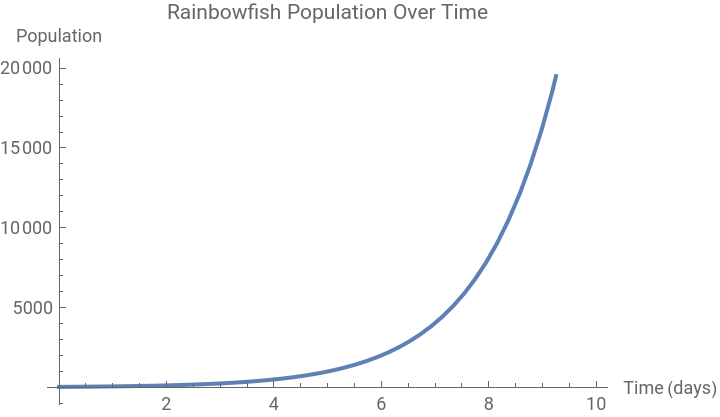
It is not realistic . Because after of a period of time we will have overpopulation of rainbow fish
First case
First case
In[]:=
Clear["Global`*"]
◼
In this section we will add one sentence to our problem, in hope that this will limit the growth
“The aquarium owner expects to sell 20 rainbowfish everyday”
Now, 20 fish per day are sold so the balance equation becomes
ΔP0.7P(t)Δt-20Δt
If we use the above equation, our differential equation will become
′
P
In[]:=
eqn={P'[t]==0.7*P[t]-20}
Out[]=
{[t]-20+0.7P[t]}
′
P
In[]:=
cond={P[0]==30}
Out[]=
{P[0]30}
In[]:=
sol=DSolve[{eqn,cond},P[t],t]
Out[]=
{{P[t]1.42857(20.+1.)}}
0.7t
In[]:=
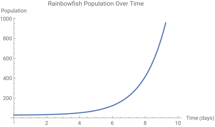
Plot[P[t]/.sol,{t,0,10},AxesLabel->{"Time (days)","Population"},PlotLabel->"Rainbowfish Population Over Time"]
Out[]=
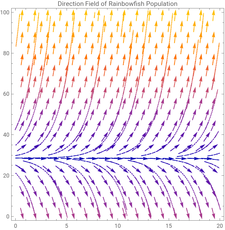
How you can construct the direction field of our differential equation and how you can sketch solutions to the differential equation if you know the initial condition
If we calculate the rates of change for many population sizes P and different times t, we can sketch the direction field.
In[]:=
VectorPlot[{1,0.7y-20},{x,0,20},{y,0,100},Axes->True,AxesLabel->{"Time (days)","Population"},StreamPoints->Fine,StreamScale->Small,PlotLabel->"Direction Field of Rainbowfish Population"]
Out[]=
Now we plot the direction field for
P(0)10,P(0)20,P(0)30,P(0)40,P(0)50,P(0)60
In[]:=
initialConditions={10,20,30,40,50,60};Show[VectorPlot[{1,0.7y-20},{x,0,20},{y,0,70},Axes->True,AxesLabel->{"Time (days)","Population"}],Plot[Evaluate[Table[NDSolveValue[{P'[t]==0.7P[t]-20,P[0]==ic},P[t],{t,0,20}],{ic,initialConditions}]],{t,0,20},PlotLegends->initialConditions,PlotStyle->Thickness[0.005]]]
Out[]=
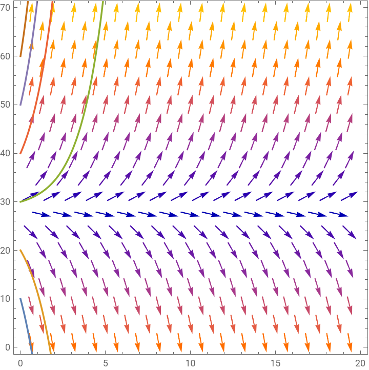


Here the equilibrium point is 20/0.7
The solutions are not realistic, because if you start with 30 rainbowfish, the population grows within four days to more than a sixty rainbowfish . This number keeps increasing, which means at some time the aquarium will be really full (and might even break)
Second case
Second case
◼
In this section, we will incorporate the limited capacity of the aquarium. When an aquarium gets crowded, the fish lay fewer eggs, fewer young fish survive and the fish may die earlier, so the growth of the population slows down.
The problem statement is now :
An aquarium owner is breeding a population of rainbowfish . He starts with 30 rainbowfish and expects to sell 20 rainbowfish every day . The aquarium is large enough for a healthy population of 750. Predict the development of the size of the population .
An aquarium owner is breeding a population of rainbowfish . He starts with 30 rainbowfish and expects to sell 20 rainbowfish every day . The aquarium is large enough for a healthy population of 750. Predict the development of the size of the population .
So the mathematical model has to be improved to be more realistic
So the differential equation becomes
From the direction Field we can observe that 720.248 is stable and 29.7516 is unstable.
Improving the model
Improving the model
Now we want to know how long it takes to breed them . Do you have to invest years to grow a good - sized population, or can it be done in a few weeks?
We will focus on answering the following question :
How long does it take for the rainbowfish population to get into its equilibrium state?
How long does it take for the rainbowfish population to get into its equilibrium state?
How long does it take to reach that equilibrium?
Mathematically, the answer is : "infinitely long"
Mathematically, the answer is : "infinitely long"
A possible solution is shown below .
It is much more difficult to guess how long the beginning and the end phases take .
The Euler’s Method
The Euler’s Method
As we can see both ways are quite accurate .
Problem Extension (Predators and Prey)
Problem Extension (Predators and Prey)
Rainbowfish and gouramis
Rainbowfish and gouramis
Before, we modelled the population size of rainbowfish in an large aquarium using limited growth and harvesting .
We consider the following problem :
A client of the fish farm wants an aquarium containing both rainbowfish and gouramis . The client is advised that the particular kind of gouramis he wants, can get aggressive, and that they hunt and eat rainbowfish . The client is undaunted and still wants this combination . He has a budget for 20 rainbowfish, 5 gouramis and an aquarium which has a maximum capacity for 100 rainbowfish . Is it possible to have both fish in the same aquarium without one of them going extinct?
We will construct a system of differential equations for interacting population :
◼
Aquarium without gouramis
◼
Aquarium without Rainbowfish
◼
Now we put the 5 gouramis and the 20 rainbowfish in the same tank.
The gouramis population will benefit from eating rainbowfish, so a positive term should be added to the following equation
or we could say that because the gouramis eat the rainbowfish, they die later.
Suppose each gouramis eats 4% of the rainbowfish per day and every 5 rainbowfish a gourami eats, one extra gourami is gained, so
So our equations are:
Now we want to calculate the equilibrium points
Given the system of equations :
For equilibrium points, we have :
In[]:=
Substituting these conditions into the system of equations gives :
Let' s solve for the equilibrium points :
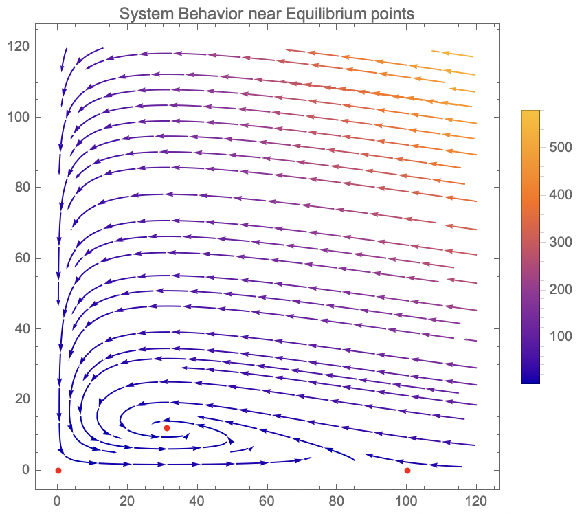
According to the model, both populations start out to grow fast to three times their initial sizes . Then first the number of rainbowfish decreases again, and the gouramis follow 6 days later . Both populations keep oscillating in a damped oscillation, and in a month or so both populations have settled in their end states of approximately 31 and 12 fishes respectively .
We are going to investigate this problem further to understand the model better
We are going to investigate this problem further to understand the model better
What would happen with different initial numbers of both kinds of fish?There are three equilibrium points . One is the end state . What is going to happen with the populations when we start near one of the other equilibrium points?Can we calculate some results analytically, so we can understand better how the parameters we have chosen for the model influence the results?And maybe then we have more information to choose realistic values for the parameter
You can see special things happening near the equilibrium points . For example near the point (100, 0), you can see lines going first towards and then away from the equilibrium .
The first step in obtaining a prediction of the behavior near the equilibrium point to find the linearization of the given system of differential equations around the equilibrium point, we need to find the Jacobian matrix and evaluate it at the equilibrium point
Find Equilibrium Points :
Compute Jacobian Matrix :
Analyze Eigenvalues :
Inspect the eigenvalues to determine the stability of the equilibrium points .
Let' s explore all the Equilibrium Points
Let' s explore all the Equilibrium Points
1
.
2
.
3
.
CITE THIS NOTEBOOK
CITE THIS NOTEBOOK
Unveiling population dynamics: from simple aquarium scenarios to complex differential equation model
by Athanasios Paraskevopoulos
Wolfram Community, STAFF PICKS, August 25, 2023
https://community.wolfram.com/groups/-/m/t/2998152
by Athanasios Paraskevopoulos
Wolfram Community, STAFF PICKS, August 25, 2023
https://community.wolfram.com/groups/-/m/t/2998152