Generalizing biological evolution, including concepts like genetic drift and selection, into a graph representation will provide a new perspective on this well established field. A general model has the potential to be expanded with new ideas, integrate many existing ones and generate predictions that can be verified empirically.
The model presented here consists of multiple types of graphs that are combined into an evolution graph. Mutation graphs represent valid changes from one genotype to another based on the underlying mutations. Fitness graphs show the fitness of these genotypes, with edges pointing towards fitter vertices. In both of these graphs the vertices are genotypes and the edges represent relationships. However, they can each be changed such that vertices are generations of a population with edges representing the changes from generation to generation. This creates a generation graph from a mutation graph that represents genetic drift (addition of genotypes by mutation), and a selection graph from the fitness graph that represents selection (removal of genotypes due to being outcompeted by fitter genotypes) . Combining the generation and selection graph creates an evolution graph that shows how generations will change based on its genotypes’ underlying mutations and fitness.
Given a specific number of genotypes it is possible to generate all its possible mutation and fitness graphs and the resulting evolution graphs. This shows patterns among the evolution graphs and makes it possible to consider the specific fitness graphs, for example ones that show epistasis, where genes interact with one another.
Two refinements of the project are the inclusion of sexual reproduction and thus recombination, and the expansion to model larger fitness graphs, by not visualizing everything as this is very computationally expensive. However there are many other questions to be asked with regards to the analysis of the evolution graphs, whether speciation is visible, and if the graphs can be used to model cross species competition.
Note: Find the complete code here
Motivation, Goal and Background
Motivation, Goal and Background
Three little birds are singing sweet songs ... but one of them is red and one of them is green and one of them is blue. Not as poetic, but important to their survival. In the long term, this survival is representative of evolution. Mutation, the possible feather colors, and fitness, the survival chances, result in “descent with modification”, a common definition of evolution because only fit animals can have offspring and mutations are necessary to create the diversity to select from (Endler, 1987).
Returning to the birds, each of them might have any color offspring. But the red bird is really obviously visible in the green forest and thus is eaten by birds of prey, the blue one is less obvious and the green one just blends in perfectly. As a result, the red bird will die before producing offspring. And after some time the bird population will consist of mostly green birds.
While this is clearly a simplification of the reality of biological evolution (for example it does not yet consider sexual reproduction and thus recombination), it lends it self as a model that utilizes graph theory for the formalization of evolutionary concepts. Not only can mathematical ideas such as eigenvalues and vectors, sinks and sources and graph distances be used, but the visualization of descent and generational changes is also an attractive quality of this approach.
Using graphs in biological evolution isn’t a new concept. Phylogenetic trees visualize long term evolution and pedigrees show the inheritance of traits, like genetic diseases. Evolutionary graph theory considers individuals to inhabit vertices and edge weights to determine fitness. A different notion, which turned out to be key to this project is that of fitness graphs where a fitness function is represented in a graph (Kaznatcheev, 2019). But more on that in a bit.
Mutations, Generations and Genetic Drift
Mutations, Generations and Genetic Drift
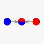
Lets return to the birds and visualize the example. If each genotype (red, blue or green) is a vertex, then edges indicate possible mutations. If each bird can have offspring of any color, then the mutation graph will look as follows:
In[]:=
mutationgraph=ColorGraph[{RedBlue,BlueGreen,GreenRed}]
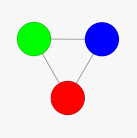
A biological side note: if the genotypes represent the actual color of the birds’ feathers, then technically they are phenotypes, because they are visible traits, but they don’t have to be the actual colors, so I will continue to refer to them as genotypes.
An alternative way of representing these genotypes is through generation vectors. This idea came from unrolling the mutation graph into a multiway system and foliating it. Each leaf of a foliation turns out to be a generation vector (please refer to the complete notebook for a more detailed explanation - link will be added as soon as its available).
Each generation vector is a list of the genotypes present in a given generation. If it happens to be the case that there are only red birds and then they produce offspring and some of them turn out to be blue, and then the blue and the red birds create some blue, red and green birds, then the generation vectors would be as follows:
Each generation vector is a list of the genotypes present in a given generation. If it happens to be the case that there are only red birds and then they produce offspring and some of them turn out to be blue, and then the blue and the red birds create some blue, red and green birds, then the generation vectors would be as follows:
In[]:=
Red{Red,Blue}{Red,Blue,Green}
Out[]=


However, this is not the only way the generations could update. What changes in generations are valid depends on the underlying mutation graph. A generation graph, where each vertex is a generation vector, helps visualize all possible changes based on a mutation graph. Edges are additions of genotypes to a generation due to mutation.
In[]:=
mutationgraphGenerationGraph[mutationgraph]
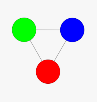
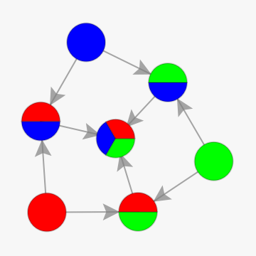
This graph shows that all mutations eventually go to a generation of birds of all colors, which simply implies that once all three colors are established, it is really unlikely to lose one of them again purely due to genetic drift.
Fitness and Selection
Fitness and Selection
It has already been established that genetic drift isn’t enough for evolution, selection is necessary too. This is where the afore mentioned fitness graphs come in. Their concept is very similar to that of the mutation graphs. Each vertex is a genotype, edges are directed at the more fit genotype. So in the example from before, green out competing blue, out competing red, would look as follows:
In[]:=
fitnessgraph=ColorGraph[{RedGreen,RedBlue,BlueGreen}]
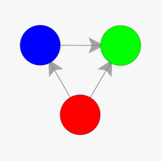
And you might have guessed that these changes can be shown on a generational level too, except that here they represent selection. So losing, red and then blue, might look something like this:
In[]:=
{Red,Green,Blue}{Green,Blue}{Green}
Out[]=
,,,
And generalized into a selection graph, which indicates the removal of genotypes because they are outcompeted by more fit genotypes:
In[]:=
SelectionGraph[fitnessgraph]
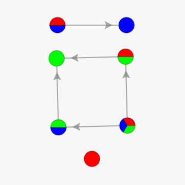
This graph implies that we will never select for red, except when there are only red birds, that green is the local sink (a generation compositions that selection pushes a population into) for any generation that has a green population, and blue is the local sink for a population with no green but some blue birds.
Evolution
Evolution
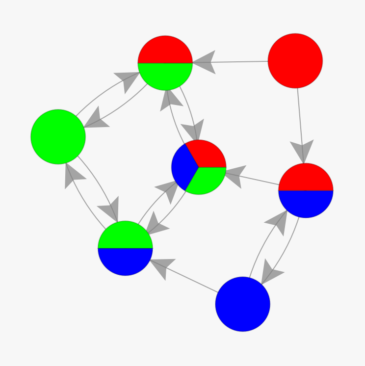
The truly exciting part is combining these two things to generate an evolution of the bird population. For that, the generation graph and the selection graph are simply combined.
In[]:=
EvolutionGraph[mutationgraph,fitnessgraph]
In[]:=
GraphSinks[EvolutionGraph[mutationgraph,fitnessgraph]]
Out[]=
{}
In[]:=
GraphSources[EvolutionGraph[mutationgraph,fitnessgraph]]
Out[]=
The graph shows that a stable population of only red birds is not possible, which is also reflected in the fact that it is a graph source (generations that the population moves away from due to selection). There is no single stable generation that the population will become (no graph sinks) because selection isn’t strong enough here to completely outweigh the effect of mutation. This is in part because of underlying assumptions of the model, which until now don’t weigh the rarity of mutation and the strength of selection.
Explorations, Epistasis, and P. Falciparum
Explorations, Epistasis, and P. Falciparum
Two Genotype Systems
Two Genotype Systems
In order to gain an initial idea of the possibilities that this model carries, let us consider a model with only two genotypes (red or blue). After generating all possible fitness graphs (f), and mutation graphs (m), their combination creates the following evolution graphs:
In[]:=
evoGrid=Table[EvolutionGraph[x,y],{y,fitgraphs},{x,mutgraphs}];Grid[Prepend[MapThread[Prepend,{evoGrid,fitgraphs}],Prepend[mutgraphs,Item[Grid[{{},{"","","m"},{},{"f","",""}}],Alignment{Bottom,Right}]]],Dividers{{False,True},{False,True}}]
Out[]=
| |||||||||||||||
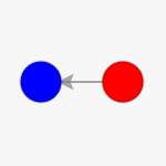
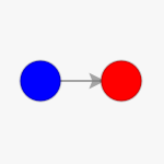
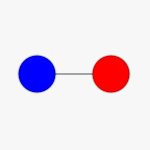
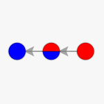
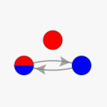
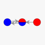
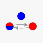
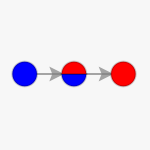
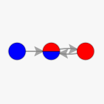
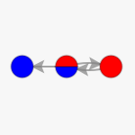
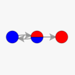
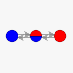
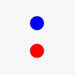
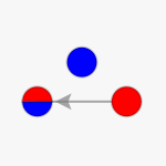
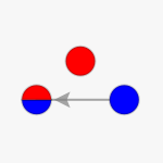
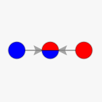
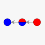
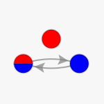
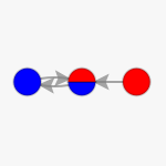
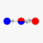
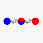
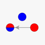
Since the mutation and fitness graphs in this example carry great symmetry, the resulting evolution graphs also look very similar. Based on an analysis of the graph’s sources, sinks, diameter, radius and distances, nine unique graphs emerge:
In[]:=
IsomorphicGraphRepresentatives[Flatten[Table[EvolutionGraph[x,y],{y,fitgraphs},{x,mutgraphs}]]]
Out[]=
,
,
,
,
,
,
These graph’s sinks can also be analyzed explicitly (not that finding the unique graphs includes picking out the first of an isomorphic group, so blue is not more dominant, it is just represented more in these graphs):
In[]:=
Row[Column[{#,Row[GraphSinks[#]," "]},AlignmentCenter]&/@IsomorphicGraphRepresentatives[Flatten[Table[EvolutionGraph[x,y],{y,fitgraphs},{x,mutgraphs}]]]," "]
Out[]=
|

|

|
|
|
|
|
Alternatively a specific mutation graph can be selected and all evolution graphs based on all possible fitness graphs can be generated and analyzed:
Three Genotype Systems
Three Genotype Systems
These analyses can be expanded to larger mutation and fitness graphs, although due to the rendering of the visualizations this becomes very computationally expensive - something to work on.
Here is a snippet of a table of evolution graphs similar to the one above but with three genotypes:
Here is a snippet of a table of evolution graphs similar to the one above but with three genotypes:
Epistasis and P. falciparum
Epistasis and P. falciparum
Another possible use of this model is to model real life data. The Kaznatcheev (2019) paper uses fitness graphs to analyze real life systems that exhibit epistasis (interaction of genes that affects the expression of the gene and thus the genotype). One of the examples they use is P. falciparum, which has the following fitness graph:
Part of the complexity of this graph is seen in the fact, that it has two unique local sinks:
Unfortunately, the model code is not yet optimized enough to generate the evolution graph (which would have over 65 500 vertices), even when the graph is not printed. For now, we can look at the effect of different forms of epistasis in simpler systems though.
In these models each genotype consists of two genes (a and b), which can be expressed as a small or capital letter. Epistasis is the interaction of two genes and where the specific expression of the gene impacts the genotype. The standard fitness graph is as follows and implies that when there is no interaction then the genotype with a capital expression is fitter than that with a small expression. So A>a, B>b, thus AB>{Ab,aB}>ab.
In these models each genotype consists of two genes (a and b), which can be expressed as a small or capital letter. Epistasis is the interaction of two genes and where the specific expression of the gene impacts the genotype. The standard fitness graph is as follows and implies that when there is no interaction then the genotype with a capital expression is fitter than that with a small expression. So A>a, B>b, thus AB>{Ab,aB}>ab.
But if the expression of b, as b or B, impacts the expression of a, then that also impacts the fitness. The following example is called sign epistasis because the expression of b as a small b reverses the fitness relationship between a and A:
The other possibility is for there to be reciprocal sign epistasis, which occurs when both gene’s fitness with respective to it alternative expression depends on the others expression:
Assuming only single point mutations to be possible (so within one mutation it is not possible to change the expression of both a and b), the mutation graph for these systems would look as follows:
This allows for an analysis of the evolution graphs and the graph’s sources (generations that the population moves away from due to selection) and sinks. None of the evolution graphs have any sinks and sign epistasis does not impact the graph’s sources, but reciprocal sign epistasis does.
Future Directions
Future Directions
A lot is still to be explored, from considerations of what a “generation level fitness graph” might be to the inclusion of sexual reproduction and thus recombination. Establishing this model is only the first step, there is room for improvement, and the analysis above is more so a proof of concept than something complete. Questions I have for myself and these models include: What do evolution graph eigenvectors mean biologically? How exactly does epistasis manifest? Can speciation be observed when sexual recombination is included? What results do these models predict for real life populations? Can the models be used to analyze cross species competition and things like symbiosis or parasitism?
Keywords
Keywords
◼
Graphs
◼
Evolution
◼
Biology
◼
Multiway Systems
Acknowledgment
Acknowledgment
Mentor: Taliesin Beynon
I would like to thank Taliesin Beynon for creating the model’s assumptions and logical underpinnings, including the relationships between all the different graphs, together with me. I am also grateful for Stephen Wolfram and the summer school for giving me the opportunity to work on this project, and Nikolay Murzin for rescuing the graph pies. Thank you to Stephen Wolfram, Taliesin Beynon, and Jonathan Gorard for coming up with the outline of this project.
References
References
◼
Kaznatcheev, A. (2019). Computational Complexity as an Ultimate Constraint on Evolution. Genetics, 212(1), 245-265. https://doi.org/10.1534/genetics.119.302000
◼
Endler, J. (1986). Natural Selection in the Wild. Princeton, NJ: Princeton University Press.