In Reference [4], Discrete damped harmonic oscillator, we applied early discretization to the damped harmonic oscillator (DHO). The discrete solution compared favorably to the standard analytical solution. Later, in Reference [5], Perspectives on energy conservation: discrete variational spherical pendulum, we discovered undesirable periodic energy error in the discrete solution, error that grows and accelerates, error that we didn’t look for first-time-around. Long-term mean energy conservation was excellent, as expected from the mathematics, but the periodic error was troubling.
Amongst the obvious new questions are “Do all discrete solutions in classical mechanics show such energy noise, or only more complex problems like the spherical pendulum?” “Can we quantify the error and characterize it qualitatively?”
Here, we launch some new notebooks to study energy noise in discrete dynamics. The DHO shows periodic energy noise of RMS that scales downward with the time step in the logarithm. When time step is , RMS error is around ; time step , RMS error around ; and so on.
Amongst the obvious new questions are “Do all discrete solutions in classical mechanics show such energy noise, or only more complex problems like the spherical pendulum?” “Can we quantify the error and characterize it qualitatively?”
Here, we launch some new notebooks to study energy noise in discrete dynamics. The DHO shows periodic energy noise of RMS that scales downward with the time step in the logarithm. When
log
10
-2
log
10
-4
log
10
-3
log
10
-6
Analytical Solution
Analytical Solution
In[]:=
ClearAll[L,F,V,T,Ld];
Lagrangian
Lagrangian
Potential Energy
Potential Energy
entailing spring constant κ as a free variable:
In[]:=
V[q_]:=κ
1
2
2
q
Kinetic Energy
Kinetic Energy
entailing mass as a free variable:
m
In[]:=
T[v_]:=m;
1
2
2
v
Lagrangian
Lagrangian
In[]:=
L[q_,v_,t_]:=T[v]-V[q]
Modified Euler-Lagrange Equation
Modified Euler-Lagrange Equation
t
∂L
∂v
∂L
∂q
∂F
∂v
(
1
)First Term
First Term
We correct the first term, a total time derivative, an explicit constant-mass rule for this problem.
In[]:=
Dt[D[L[q,v,t],v],t]/.{Dt[m,t]->0}
Out[]=
mDt[v,t]
Second Term
Second Term
Partial derivative of with respect to generalized coordinate .
L
q
In[]:=
D[L[q,v,t],q]
Out[]=
-qκ
Force Term
Force Term
Choose Rayleigh's Dissipation Function, , with , the dissipation constant as a third free variable:
F=
b
2
2
v
b
In[]:=
F[q_,v_,t_]:=
b
2
2
v
Sum of all Terms
Sum of all Terms
In[]:=
deqn=deqn=((Dt[D[L[q,v,t],v],t]-D[L[q,v,t],q]+D[F[q,v,t],v])/.{Dt[m,t]->0}/.{v->Dt[q,t]}/.{q->x[t]})==0
Out[]=
κx[t]+b[t]+m[t]0
′
x
′′
x
Analytical Solution
Analytical Solution
Pick the pertinent part of the expression returned by DSolve:
In[]:=
asoln=(DSolve[deqn,x,t])[[1,1,2]]
Out[]=
Function{t},t---4mκ+t-+-4mκ
1
2
b
m
2
b
m
1
1
2
b
m
2
b
m
2
Numerical Rules
Numerical Rules
For all subsequent plots and demonstrations, choose the following values for the constants .
κ,m,C[2],C[1]
In[]:=
ClearAll[numRules];numRules={κ->1,m->1,C[2]->1,C[1]->0};
Plot
Plot
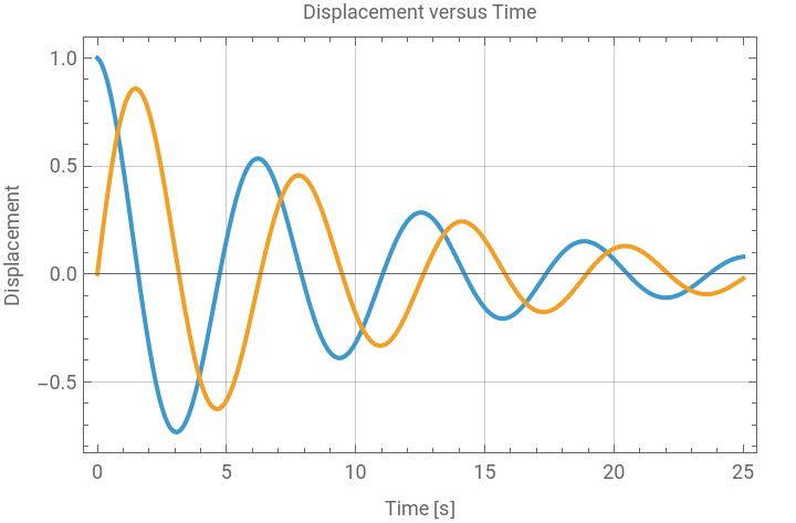
Over 25 seconds’ time, plot the displacement; tLim=25 is a constant over all the plots in this notebook:
In[]:=
tLim=25;
If is smaller than , we get complex exponentials. Only the real parts are physical, but we plot the imaginary parts for mathematical interest.
2
b
4mκ
As varies from 0 to , the system transitions from undamped and purely sinusoidal, to underdamped showing oscillation, to critically damped when the imaginary part goes to zero, to overdamped showing no oscillation. See this page on damping.
2
b
4mκ=4
In[]:=
Manipulate[Plot[{Re[asoln[t]]/.numRules/.{b->bManip},Im[asoln[t]]/.numRules/.{b->bManip}},{t,0,tLim},GridLines->Automatic,PlotLegends->{"Real Part","Imaginary Part"},GridLines->All,Frame->True,FrameLabel->{{"Displacement",""},{"Time [s]","Displacement versus Time"}}],{{bManip,0.2},0,4,Appearance->"Open"},SaveDefinitions->True]
Out[]=




Analytical Energy
Analytical Energy
We need generalized velocity via a new, “dummy” differentiation variable, , to avoid collision with plotting variable :
u
t
In[]:=
D[asoln[u],u]
Out[]=
1
2
1
2
b
m
2
b
m
b
m
2
b
m
1
1
2
1
2
b
m
2
b
m
b
m
2
b
m
2
Take only the real parts. Don’t be tempted to take the magnitude of a complex-valued energy! It mixes in the non-physical imaginary part.
In[]:=
ClearAll[analyticalEnergy];analyticalEnergy[t_]:=V[Re[asoln[t]]]+T[Re[D[asoln[u],u]]]/.{u->t};
In[]:=
Manipulate[Plot[analyticalEnergy[t]/.numRules/.{b->bManip},{t,0,tLim},GridLines->All,Frame->True,FrameLabel->{{"Energy [J]",""},{"Time [s]","Analytical Energy versus Time"}}],{{bManip,0.2},0,4,Appearance->"Open"},SaveDefinitions->True]
Out[]=
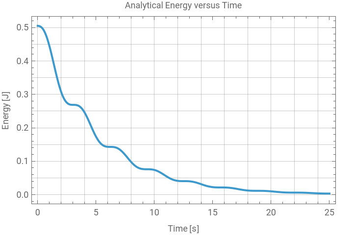
Notice that the energy is conserved only when , at critical damping, but not otherwise. Such is expected from the physics: the DHO is a non-conservative system. Near critical damping , no “bumpy” structure is seen.
b=2
b=2
Discrete Solution
Discrete Solution
Reference 2 gives us the forced discrete Euler-Lagrange Equations:
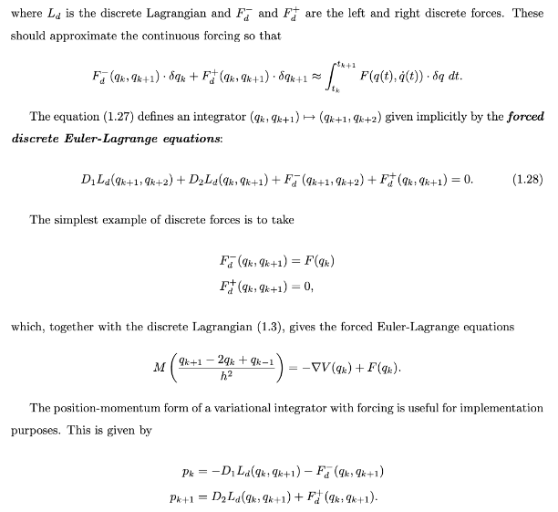
Guess that the discrete generalized forces are derivatives of the damping force. This guess does not introduce risky physics because we can always check the undamped case. In other cases, the results are so plausible that we are satisfied with the guess.
and write
Pick the solution out of Wolfram’s structure and apply the arithmetic rules:
Compare Solutions
Compare Solutions
Displacement
Displacement
Wolfram could not solve the recurrence exactly within a few minutes. However, I left the expression in an unevaluatable cell in case you’d like to try it.
We’ll settle for a direct, brute-force evaluation of the recurrence.
Energies
Energies
We need velocities for kinetic energy.
The discrete solution tracks the analytical solution fairly well, at least visually. However, the energy difference shows periodic structure for all damping constants and time steps.
The RMS energy error shows a peak at critical damping, and interesting structure for other damping constants.
Conclusion
Conclusion
The damped harmonic oscillator shows periodic energy noise at all values of the damping constant and time step that we tried. The energy noise peaks at critical damping. It scales downward with time step in an approximate linear relationship in the logarithms.
This is good news and bad news. The good news is that the noise is manageable. The bad news is that we don’t fully understand it and we can’t make it go away. This is surprising given that the mathematics is purported to have the best possible energy behavior amongst all integration schemes because it follows the natural Lie-group structure of the problem. We must keep digging to understand the origin of this noise.
We also note that the run-time speed of the discrete method is too slow. We have work to do to speed it up.
References
References
1
.Marsden and West, 2001, Discrete Mechanics and Variational Integrators, http://www.cds.caltech.edu/~marsden/bib/2001/09-MaWe2001/MaWe2001.pdf
2
.Matthew West, Variational Integrators, Caltech Thesis, May 2004, https://thesis.library.caltech.edu/2492/1/west_thesis.pdf
3
.Marin Kobilarov and Jerrold E. Marsden, Discrete Geometric Optimal Control on Lie Groups, IEEE Transactions on Robotics, Vol. 27, No. 4, August 2011.
4
.Discrete damped harmonic oscillator
by Brian Beckman
Wolfram Community, STAFF PICKS, May 13, 2024
https://community.wolfram.com/groups/-/m/t/3174169
by Brian Beckman
Wolfram Community, STAFF PICKS, May 13, 2024
https://community.wolfram.com/groups/-/m/t/3174169
6
.Energy perspectives on the discrete harmonic oscillator, Brian Beckman, April 2025, to appear.
CITE THIS NOTEBOOK
CITE THIS NOTEBOOK
Energy perspectives: discrete damped harmonic oscillator
by Brian Beckman
Wolfram Community, STAFF PICKS, April 20, 2025
https://community.wolfram.com/groups/-/m/t/3447615
by Brian Beckman
Wolfram Community, STAFF PICKS, April 20, 2025
https://community.wolfram.com/groups/-/m/t/3447615