Bullvalene is an interesting polycyclic hydrocarbon that was first hypothesized by Doering and Roth in 1963, and then subsequently synthesized by Schröder in 1963. It is an example of a "fluxional molecule", a molecule where the bonds migrate at a rate such that all the atoms are symmetry-equivalent (in room temperature, at least). When one takes the proton NMR spectrum of bullvalene, one would only find a single peak.
More precisely, bullvalene undergoes a Cope rearrangement, a special type of pericyclic reaction where a single bond in a 1,5-diene moves three atoms away from its starting point at both ends (that is, a [3,3]-sigmatropic rearrangement). The result is that bullvalene can rearrange itself into any of 10!/31209600 equivalent structures. (For further details on bullvalene and its story, see Ault's article.)
Here’s a bullvalene molecule, generated from its SMILES representation. (In preparation for further manipulations to be done later, let’s automatically generate 3D coordinates for it using MoleculeModify[“ComputeAtomCoordinates”]):
In[]:=
bullvalene=Molecule["C\\2=C\\C/1\\C=C/C3C(\\C=C\\1)C/23"]//MoleculeModify["ComputeAtomCoordinates"]
Out[]=
Molecule


In[]:=
bullvalene//{MoleculePlot,MoleculePlot3D}/*Through/*GraphicsRow
Out[]=
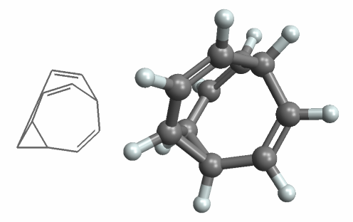
I wanted to simulate the fluxional property of bullvalene through its 3D depiction. To do that, I constructed a MoleculePattern corresponding to a 1,5-diene substructure:
In[]:=
(*MoleculePattern["C=CCCC=C"]*)patt=MoleculePattern[{"C","C","C","C","C","C"},{Bond[{1,2},"Double"],Bond[{2,3},"Single"],Bond[{3,4},"Single"],Bond[{4,5},"Single"],Bond[{5,6},"Double"]}]
Out[]=
MoleculePattern

For bullvalene itself, this substructure occurs thrice. We can use MoleculeSubstructureCount to count the occurrences, and MoleculePlot3D to depict them:
In[]:=
MoleculeSubstructureCount[bullvalene,patt]
Out[]=
3
In[]:=
MoleculePlot3D[bullvalene,patt]
Out[]=

One way to implement the Cope rearrangement involves the use MoleculeModify[“ReplaceSubstructure”] to change the bonding within a molecule. As a demonstration of what happens in a Cope rearrangement, let’s do it on a simpler hydrocarbon (the migrating bond is highlighted in both the starting material and product):
In[]:=
before=Molecule["3-methyl-1,5-hexadiene"];repl=Molecule[{"C","C","C","C","C","C"},{Bond[{1,2},"Single"],(*swapsinglesfordoubles*)Bond[{2,3},"Double"],Bond[{1,6},"Single"],(*removethe3-4bond,adda1-6bond*)Bond[{4,5},"Double"],Bond[{5,6},"Single"]}];after=MoleculeModify[before,{"ReplaceSubstructure",Values[FindMoleculeSubstructure[before,patt][[1]]]->repl}];{MoleculePlot[before,Bond[{3,4}],IncludeHydrogens->None],Graphics[{Arrowheads[Large],Arrow[{{0,0},{2,0}}]}],MoleculePlot[after,Bond[{5,10}],IncludeHydrogens->None]}//GraphicsRow
Out[]=

With all required pieces in place, here is a function that will randomly transform a bullvalene molecule into another (equivalent!) arrangement:
In[]:=
newbull[bull_]:=Module[{subl},subl=Values[RandomChoice[FindMoleculeSubstructure[bull,patt,All]]];MoleculeModify[MoleculeModify[bull,{"ReplaceSubstructure",subl->repl}],"EnergyMinimizeAtomCoordinates"]]
MoleculeMatchQ can be used to confirm that the result of the transformation is still bullvalene, even after shuffling the bonds:
In[]:=
MoleculeMatchQ[bullvalene,newbull[bullvalene]]
Out[]=
True
Generate a few frames of the simulation (we use PlotTheme”HeavyAtom” to suppress hydrogen atoms in the depiction, which would only clutter the simulation):
In[]:=
blist=NestList[newbull,bullvalene,25];frames=MoleculePlot3D[#,PlotTheme->"HeavyAtom",ViewPoint{-1.41,0.1,-3.1}]&/@blist;
In[]:=
ListAnimate[frames,AnimationRunning->False]
Out[]=

Acknowledgements
I would like to thank Jason Biggs for helping me streamline some of the code used in this post.
I would like to thank Jason Biggs for helping me streamline some of the code used in this post.
CITE THIS NOTEBOOK
CITE THIS NOTEBOOK
Coping with Bullvalene's Rearrangements
by J. M.
Wolfram Community, STAFF PICKS, December 20, 2023
https://community.wolfram.com/groups/-/m/t/3087883
by J. M.
Wolfram Community, STAFF PICKS, December 20, 2023
https://community.wolfram.com/groups/-/m/t/3087883