This is a notebook where I try to use Mathematica and its Neural Networks framework to solve PDE problems (in this case Laplace equation on an L-shaped domain). At present (2022, Mathematica 13.0), the lack of an Auto-Differentiation algorithm (like that internal of TensorFlow) is avoided using a native definition of Derivative for a net. In this way, using Mathematica internal Function NetArray in the definition of a net, the trained Weights and Biases are hereditated by its Derivatives during training.
All suggestions for better results are welcome! Many thanks.
Gianluca
All suggestions for better results are welcome! Many thanks.
Gianluca
This is a Function to create automatically a Neural Network with
neurons = number of elementary neurons per layer
level = total number of layers for the net
activationFun = the activation function at the end of the layers
finalFun = a one-dimensional function for a single output at the end of the net
s = a letter for identification of Weights and Biases for every net, in the case of multiple nets
layersList[s_String,neurons_Integer,activationFun_,level_Integer,finalFun_]:={Flatten[AppendTo[(#;{LinearLayer[neurons,"Weights"NetArray[StringJoin[s,"W",ToString[#]]],"Biases"NetArray[StringJoin[s,"B",ToString[#]]]],activationFun})&/@Range[1,level],{CatenateLayer[],finalFun,LinearLayer[1,"Weights"NetArray[StringJoin[s,"W",ToString[level+1]]],"Biases"NetArray[StringJoin[s,"B",ToString[level+1]]]]}],1],{k=1;listTemp={};Do[(AppendTo[listTemp,k->k+1];k=k+2),{m,1,level}];Sequence@@listTemp,(2*#)&/@Range[1,level]->2*level+1->2*level+2->2*level+3}}
The L-shaped domain
domain=Region[RegionDifference[Rectangle[{-1,-1},{1,1}],Rectangle[{0,0},{1,1}]]]
Out[]=

This is the unknown net as function to be computed
Clear[u];layersList["u",64,Tanh,8,LogisticSigmoid];u=NetGraph[%[[1]],%[[2]]];
These are nets representing the Partial Derivatives of the unknown u.
Very Important: using NetArray in the definition of u net, the trained Weights and Biases are hereditated by its Derivatives during training.
Very Important: using NetArray in the definition of u net, the trained Weights and Biases are hereditated by its Derivatives during training.
sdx=0.01;sdy=0.01;udxx=With[{dx=sdx},NetGraph[{FunctionLayer[Function[#]],FunctionLayer[Apply[Function[{{#[[1]]-dx,#[[2]]},{#[[1]],#[[2]]},{#[[1]]+dx,#[[2]]}}]]],NetMapOperator[u],FunctionLayer[Function[(#[[3]]-2*#[[2]]+#[[1]])/(dx^2)]]},{1->2->3->4}]];udyy=With[{dy=sdy},NetGraph[{FunctionLayer[Function[#]],FunctionLayer[Apply[Function[{{#[[1]],#[[2]]-dy},{#[[1]],#[[2]]},{#[[1]],#[[2]]+dy}}]]],NetMapOperator[u],FunctionLayer[Function[(#[[3]]-2*#[[2]]+#[[1]])/(dy^2)]]},{1->2->3->4}]];
This is the net representing the PDE Laplace equation Δu = - 1;
The parameter represented by #[[4]] is simply a swith parameter s = 1 for training on internal points, s = 0 for boundary points.
The parameter represented by #[[4]] is simply a swith parameter s = 1 for training on internal points, s = 0 for boundary points.
pde=NetGraph[{FunctionLayer[Apply[{#[[2]],#[[3]]}&]],u,udxx,udyy,FunctionLayer[Apply[{#[[1]]}&]],CatenateLayer[],FunctionLayer[Function[#[[4]]*(#[[2]]+#[[3]])+(1-#[[4]])*#[[1]]]]},{NetPort["Input"]->{1,5},1->{2,3,4},{2,3,4,5}->6->7},"Input"->3];
5000 points for training into the domain.
internalPoints=RandomPoint[domain,5000];
2000 point for training onto the boundary.
boundaryPoints=RandomPoint[RegionUnion[{Line[{{-1,-1},{1,-1}}],Line[{{1,-1},{1,0}}],Line[{{1,0},{0,0}}],Line[{{0,0},{0,1}}],Line[{{0,1},{-1,1}}],Line[{{-1,1},{-1,-1}}]}],2000];
These are the sets of points for training; the parameter s = 1 or s = 0 is prepended to spatial coordinates
on internal points equation is trained to be -1., on boundary points u is trained to be 0.
on internal points equation is trained to be -1., on boundary points u is trained to be 0.
internalData=(PrependTo[internalPoints[[#]],1]->-1.)&/@Range[1,Length[internalPoints]];boundaryData=(PrependTo[boundaryPoints[[#]],0]->0.)&/@Range[1,Length[boundaryPoints]];pdeTemp=pde;
Training iterations
MaxIters=5;(#;pdeTemp=NetTrain[pdeTemp,Join[internalData,boundaryData],BatchSize16,Method->"ADAM"])&/@Range[1,MaxIters];pdet=pdeTemp;usol=NetExtract[pdet,2];
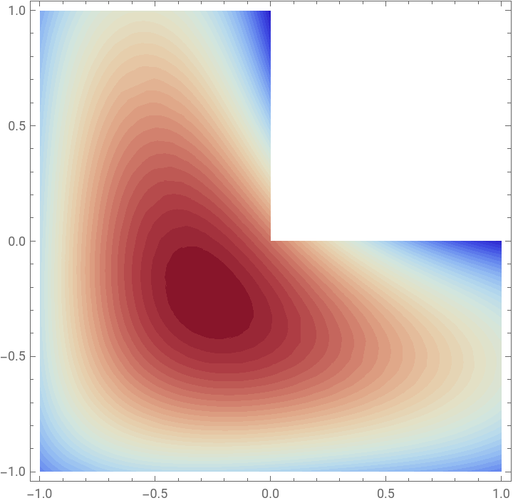
Contours plot of solution
ContourPlot[usol[{x,y}],{x,y}∈domain,Contours40,PlotRangeAll,ColorFunctionColorData["ThermometerColors"],ContourStyleNone,AspectRatioAutomatic]
Out[]=
CITE THIS NOTEBOOK
CITE THIS NOTEBOOK
PINN: Physics Informed Neural Networks for Laplace PDE on L-shaped domain
by Gianluca Argentini
Wolfram Community, STAFF PICKS, June 24, 2022
https://community.wolfram.com/groups/-/m/t/2557040
by Gianluca Argentini
Wolfram Community, STAFF PICKS, June 24, 2022
https://community.wolfram.com/groups/-/m/t/2557040