“Free will is the supposed power or capacity of humans to make decisions or perform actions independently of any prior event or state of the universe.”
In this computational essay, we explore whether artificial neural networks — trained from different random initializations — exhibit signs of computational irreducibility in their weight trajectories. We hypothesize that if networks trained to perform the same task arrive at different internal configurations, despite converging on similar outputs, this divergence may reflect irreducible computational behavior — a necessary (though not sufficient) condition for free will.
To test this, we started by training a simple three-layer feedforward neural network on a piecewise function under two different random seeds. After convergence, we compared their internal weights using the Hungarian algorithm to correct for neuron permutation invariance. Although both networks achieved similar loss values, their final weights differed measurably.
These preliminary results suggest that neural network training dynamics are path-dependent and potentially irreducible, even in simple settings. We propose that such variability in internal representations — if expanded and validated — could form the basis for exploring primitive forms of agency in artificial systems.
Introduction
Introduction
Wouldwesaythatananthasanydegreeoffreedomorgetstoexerciseitsfreedomofwillifwecanreasonablypredictitsactions?Probablynot.Whatabouthumans?Canwepredictwhatahumanagentisgoingtodobeforetheagentcarriesouttheiractionswithgreatcertainty?Probablynot.“Whilemanycomputationsadmitshortcutsthatallowthemtobeperformedmorerapidly,otherscannotbespedup.Computationsthatcannotbespedupbymeansofanyshortcutarecalledcomputationallyirreducible.Theprincipleofcomputationalirreducibilitysaysthattheonlywaytodeterminetheanswertoacomputationallyirreduciblequestionistoperform,orsimulate,thecomputation.Someirreduciblecomputationscanbespedupbyperformingthemonfasterhardware,astheprinciplerefersonlytocomputationtime.”Wepositthatasystemthathas"free will",willexhibitlotsofdifferentbehaviorsandonethatdoesnotwillexhibitveryfew.Weareinterestedinwhenneuralnets,anemulationofbiologicalthinkingprocesses,exhibitfreewill.WebaseourexperimentonDr.Wolfram'sArticle"What's Really Going On in Machine Learning"wherehesetsupmeshneuralnetworkstopredictcellularautomataandobserveshowdifferentrandomweightsaffectshisresults.Westartbychoosingamathematicalfunctionthatourneuralnetworksshallmodel.
Methodology
Methodology
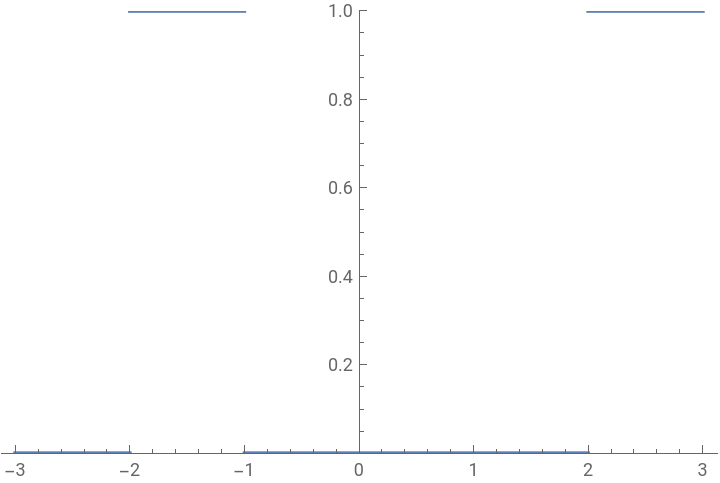
For this experiment, we wanted to choose a simple mathematical function to model and picked the piecewise function below
In[]:=
whichFunction[x_]:=Which[x<-2,0,-2<x<-1,1,-1<x<2,0,x>2,1,True,0]Plot[whichFunction[x],{x,-3,3},PlotRange->{0,1}]
Out[]=
We started by deciding on checkpoints (10,20,30,40,50,60,70,80,90% of the total training) where the weights would be saved, and a “simple” neural net architecture,with a small number of LinearLayer with a small number of neurons . Then, we initialized the net with random weights(Randomizing the seed as well as NetInitialise would otherwise use the same seed thus assigning the same weights for both the neural networks). Next,we trained 2 identical neural nets to recreate the function and recorded the number of rounds/epochs to reach convergence. It was also noted that some seeds often took more rounds to converge than others. We then stored the weights (and the final loss) in a list before resetting the weights via NetInitialise.
The next step of our experiment was retraining the 2 neural networks for 10,20,30,40,50,60,70,80 and 90 percent of the rounds we know would lead to convergence.While retraining the neural networks, we recorded the net loss and the weights. We then calculated the distance between the weights of the neural networks layer wise by implementing the Hungarian Algorithm. This allowed us to find the distance between corresponding weights even if they may be permutations of each other. Our last step was plotting our results on a line graph.
We started by generating our training data below by looping through the piecewise function from a range of -3 to +3
In[]:=
trainingDataFormatted=Table[{x}->{N[whichFunction[x]]},{x,-3,3,0.001}];
Architecture of the neural network
Architecture of the neural network
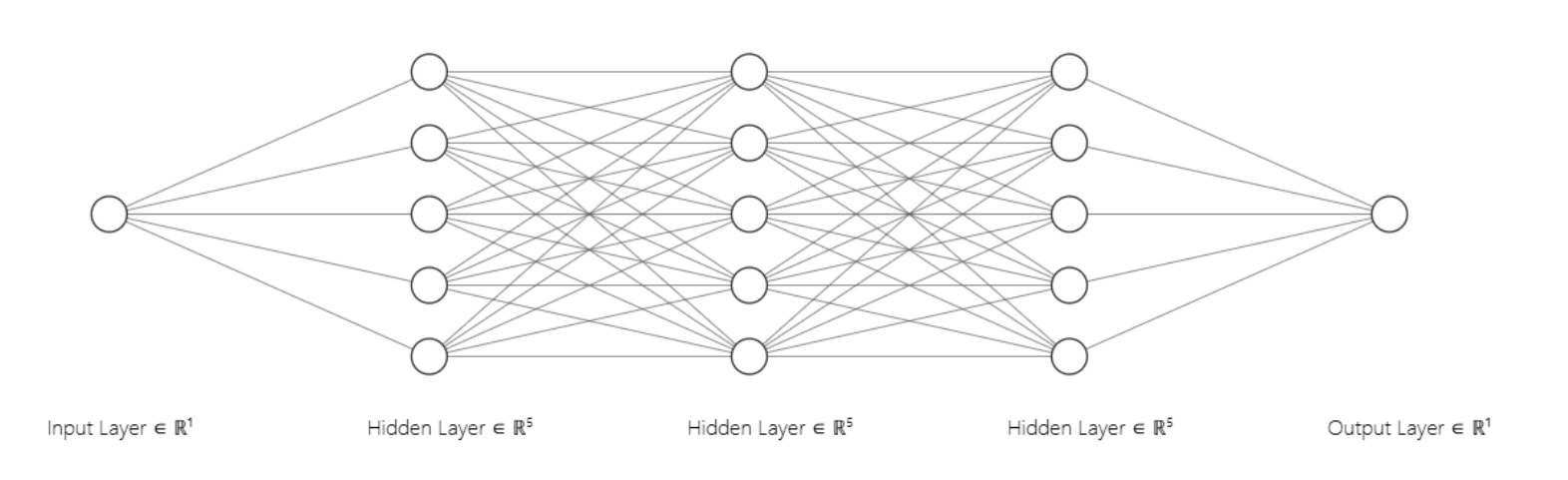
Our neural networks with 3 layers have been set up below with 5 neurons in each layer.These specific model configurations were chosen through trial and error while keeping simplicity in mind.We have chosen ReLU(Ramp) as our activation function while keeping the standard Mean squared error as our loss function. We have also chosen the Adam Optimiser to avoid getting stuck in local minima/maxima
Neural Net Implementation
Neural Net Implementation
The following cells initialize and train the neural nets.
In[]:=
newNet[]:=NetChain[{LinearLayer[5,"Input"->1],ElementwiseLayer[Ramp],LinearLayer[5,"Input"->5],ElementwiseLayer[Ramp],LinearLayer[1,"Input"->5]}]listOfNetworks=Table[newNet[],{2}]
Out[]=
NetChain,NetChain


Initialized the neural network with random weights.
Initialized the neural network with random weights.
In[]:=
initialiseNetworks[i_]:=Module[{netInitialized},netInitialized=NetInitialize[listOfNetworks[[i]],Method->{"Random"},RandomSeeding->Automatic];netInitialized]netXInitialized=Table[initialiseNetworks[i],{i,2}]
Out[]=
NetChain,NetChain

Trained the model while checkpointing the weights in a local directory. We implemented early stopping to get a more accurate estimate of the number of rounds required for our neural network to reach convergence. If there wasn’t a 0.001 change in the Mean squared error over the last 40 epochs then the neural network would stop training.
checkpointDir=CreateDirectory["checkpointoldold"]netXTrained[x_]:=Module[{trainedNetPiece},trainedNetPiece=NetTrain[netXInitialized[[x]],trainingDataFormatted,All,TrainingStoppingCriterion-><|"Criterion"->"Loss","Patience"->40,"AbsoluteChange"->0.001|>,TrainingProgressCheckpointing->{"Directory",checkpointDir,"Interval"->Quantity[1,"Rounds"]}];trainedNetPiece]
listofTrained=Table[netXTrained[i],{i,2}]
Out[]=
NetTrainResultsObject,NetTrainResultsObject

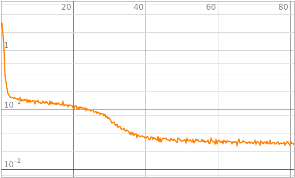
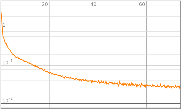
We can retrieve the number of "rounds" the model took to reach convergence
We then extract the weights of our 2 neural networks by looping through each layer of the neural network with Table and then extracting the weights with NetExtract
To calculate the distance between the weights of our neural networks, we must first sort the weights of each layer in ascending order. This is because neurons in an artificial neural network may be permutations of each other. We then Map the corresponding weights and calculate the euclidean distance between them
We can now plot the output of our trained neural nets against the objective function
We now want to repeat the training procedure but want to train each neural network for only 10,20,30,40,50,60,70,80,90% of the total number of rounds required to reach convergence. This would tell us how the weights grow closer or further apart as we train the model and if the neural networks converge or diverge at certain points of the training process.
Based on the checkpoints of the convergence times above, we retrain the neural nets below.
The line graph above shows that the weights of the neural networks do not converge but instead diverge as the euclidean distance between them increases as we train the 2 neural networks for more rounds.
Conclusion
Conclusion
This project set out to evaluate whether weights of neural networks are computationally irreducible or not as computational irreducibility is characteristic of agents who are able to exercise free will. We were able to reasonably ascertain that neural networks trained to model the same function can take various paths to do so since both of our neural networks ended up with different weights. This leads us to the conclusion that neural networks do have limited forms of free will and agency in the form of their weight trajectories, even if they are being trained to model a predefined function.
Limitations and Future Work
Limitations and Future Work
There are several limitations to the experiment we carried out. First, we intentionally chose a simple mathematical function to model. While this was useful for maintaining interpretability and reducing computational overhead, it also inadvertently simplified the loss landscape of the neural network. A less complex function typically results in smoother optimization paths and may not fully reflect the kind of chaotic or rugged training dynamics that would better demonstrate computational irreducibility.
Second, we only compared two seeds during training. While this gave us a basic sense of how different initializations can lead to different weight configurations, it is insufficient for drawing any strong statistical conclusions. Including a larger number of random seeds would have allowed us to get a clearer picture of the distribution of training trajectories and whether the observed weight divergence is a consistent phenomenon or simply a byproduct of random noise from the weight initialisation.
Third, our method of comparing weights using the Hungarian algorithm only tells us whether the final trained weights from two different networks are permutation-equivalent. While this can help us identify whether the networks converge to similar representations up to neuron order, it does not reveal whether the networks have actually diverged in a meaningful/ functionally different way. It is also difficult to distinguish between divergence caused by inherent irreducibility in the training process versus variation due to the initial randomness of weights
Given these limitations, there are several directions for future work. The first is to repeat the experiment with at least 30 different seeds, which would provide better statistical resolution and reveal the underlying variance in the optimization paths. Second, instead of a simple piecewise function, future experiments should use more complex or chaotic datasets — such as time steps of Rule 110 cellular automata — which are more likely to exhibit computational irreducibility. Third, adding dropout layers would introduce stochasticity during training, allowing us to test how sensitive the network’s behavior is to small perturbations. Finally, implementing Monte Carlo Dropout would allow us to generate multiple predictions from the same network using different dropout masks, providing a way to quantify uncertainty and functional variability.
Acknowledgements
Acknowledgements
I would like to sincerely thank my mentor, Dr.Lyman Hurd, for his consistent guidance throughout this project. I’m also grateful to the WSRP directors(Rory Foulger, Program Director,Eryn Gillam, Academic Director,Megan Davis, Academic Director) for organizing this opportunity, and to Stephen Wolfram for helping brainstorm and shape the initial idea that inspired this work.I would also like to thank the Notebook assistant for helping me debug my code.
References
References
1)Wolfram, S. (2024, August 22). What’s really going on in machine learning? Some minimal models. Stephen Wolfram Writings. https://writings.stephenwolfram.com/2024/08/whats-really-going-on-in-machine-learning-some-minimal-models/
2)Kuhn, H. W. (n.d.). Hungarian algorithm. Retrieved July 10, 2025, from https://www.hungarianalgorithm.com/hungarianalgorithm.php
3)Rowland, T. (2025, June 27). Computational irreducibility. In MathWorld–A Wolfram Web Resource. Retrieved July 10, 2025, from https://mathworld.wolfram.com/ComputationalIrreducibility.html