How does the Copernicus Weather Replay app show you hourly weather maps anywhere on Earth, all the way back to 1 January 1940 — more than two decades before the first geostationary satellite of any kind (Syncom 3, 1964) and nearly four before Europe was watched continuously from orbit (Meteosat-1, 23 November 1977)? It is not showing you a photograph. It is showing you a reanalysis — a numerical weather model rerun retrospectively over the past, gently nudged at every moment by all the observations that existed at that moment. The output is a four-dimensional dataset of the entire atmosphere, and any "satellite image" is just one slice of it. This post unpacks what that means, then shows how to do the same thing in roughly thirty lines of Wolfram Language. The companion package HistoricalWeatherWL (attached as HistoricalWeather.wl plus its sidecar ARCO.wl) reads ERA5 directly from the public ARCO Zarr store on Google Cloud through a pure-Wolfram blosc / LZ4 / byte-shuffle decoder — no Wolfram Knowledgebase gridded data, no CDS account, no external runtime. Combined with the public NASA GIBS WMS endpoint for the post-2000 imagery, it gives you a one-liner that, for any latitude / longitude / UTC datetime since 1 January 1940, returns the surface conditions, a regional weather map, and, where one exists, a real MODIS Terra true-colour image.
1. Apollo 11 from above
1. Apollo 11 from above
Open the Copernicus Weather Replay app and paste this URL into your browser:
https://weather-replay.climate.copernicus.eu/?lat=28.6&lon=-80.6&zoom=5.0&datetime=1969-07-16T13:00:00.000Z&pickLat=28.608&pickLon=-80.604
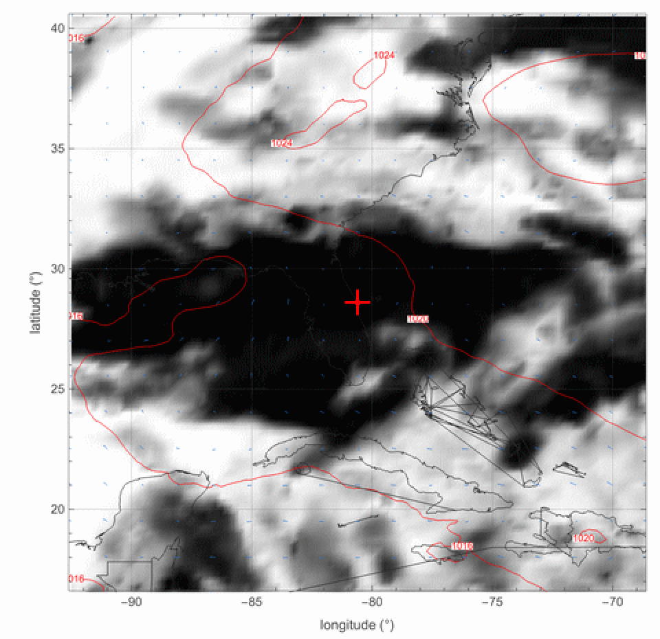
You will land on a fully animated weather map of central Florida at 13:00 UTC on 16 July 1969 — thirty-two minutes before Apollo 11 lifted off from Launch Complex 39A at Kennedy Space Center, bound for the Moon. Pick another point, scrub another hour, drag the time slider back to 1 January 1940 — it just works. The example date happens to fall inside the era of experimental geostationary imagery: NASA's ATS-3 had been transmitting spin-scan cloud pictures from a geosynchronous station over the Americas since mid-November 1967. But the archive's reach is what is astonishing: 1940 is more than two decades before Syncom 3, the first geostationary satellite of any kind, and almost four before Europe was watched continuously from orbit (Meteosat-1, 23 November 1977). So where do the maps come from?
And here is what the URL above actually returns, animated as the launch morning unfolds. Fifteen hourly synthetic-satellite frames from 06:00 to 20:00 UTC on 16 July 1969, centred on Launch Complex 39A. The Saturn V ignites at 13:32 UTC — the frame between 13:00 and 14:00 UTC straddles liftoff.
2. Reanalysis: a model run with hindsight
2. Reanalysis: a model run with hindsight
The answer is that the Weather Replay app does not play back any photograph at all. It plays back ERA5, the European Centre for Medium-Range Weather Forecasts' fifth generation atmospheric reanalysis. A reanalysis is the same numerical weather model that produces tomorrow's forecast, but run retrospectively over the historical record: at each 12-hour window the model state is brought into best simultaneous agreement with every observation that existed inside the window, then propagated forward to the next window. The result is a complete, four-dimensional picture of the atmosphere — temperature, humidity, wind, pressure, cloud on a 0.25° grid, every hour, surface to 80 km — that goes back to 1 January 1940.
2.1 Data assimilation in one equation
2.1 Data assimilation in one equation
The mathematical apparatus that fuses observations into the model state is data assimilation. ECMWF uses 4D-Var, a variational scheme that, for each 12-hour assimilation window, finds the initial state that minimises a cost function balancing two things simultaneously: how close the implied trajectory is to the prior best guess from the previous window (the background , weighted by its error covariance ), and how close it is to every observation inside the window (each weighted by its instrument-error covariance ):
x
0
x
b
B
y
t
R
J()=(-)+(-())
x
0
1
2
T
(-)
x
0
x
b
-1
B
x
0
x
b
1
2
∑
t
T
(-())
y
t
H
t
x
t
-1
R
y
t
H
t
x
t
with the model itself propagating the candidate state forward through the window,
x
t
M
0t
x
0
and the "observation operator" that maps a model state into the form of an instrument reading (a radiometer brightness, a sonde profile, a ship report, a station thermometer reading). In a purely linear, single-time idealisation the minimisation has the closed form
H
t
x
a
x
b
x
b
K=B
T
H
-1
(HB+R)
T
H
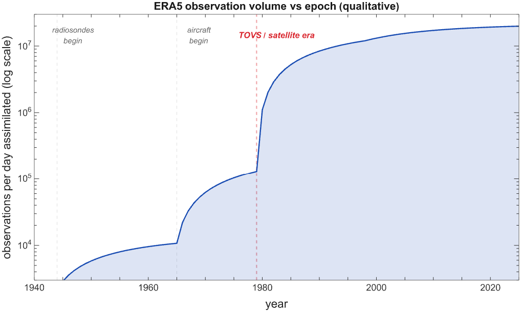
i.e. the analysis is the background plus a Kalman gain times the innovation . Where observations are dense and accurate, is large and the analysis follows the data; where they are sparse or noisy, is small and the analysis trusts the model's forecast. ERA5 streams roughly 24 million observations per day into this machinery for the modern era — and on the order of ten to twenty thousand per day for the earliest 1940s slices, drawn from surface stations, ships, and the first upper-air soundings.
K
y-H()
x
b
K
K
2.2 What was observable when?
2.2 What was observable when?
This is what makes the depth of the archive plausible. The same physics that produces a 10-day forecast can be run retrospectively on yesterday's, last decade's, or the 1940s' observations. ERA5 has surface land stations and ships of opportunity for the entire 1940–today record; it has radiosondes from the mid-1940s; aircraft reports (AIREP / PIREP from the 1960s, then AMDAR / ACARS from the late 1970s onward); and what reanalysis users call the "satellite era" — the period from early 1979 when the first TIROS Operational Vertical Sounder (TOVS) radiances entered the assimilation pool, across which the analysis quality steps up visibly in every diagnostic plot. Today's analysis also ingests geostationary radiances, scatterometer ocean winds, and GPS radio-occultation:
3. Where the data lives, and how to read it in one line
3. Where the data lives, and how to read it in one line
The reanalysis itself lives in ECMWF's ARCO ERA5 archive at gs://gcp-public-data-arco-era5 — a Zarr v2 store on Google Cloud, anonymous reads over HTTPS, no CDS account, no API key. The shape of one variable is {1323648, 721, 1440}: hours since 1900, latitudes 90−90 in 0.25° steps, longitudes 0359.75 in 0.25° steps.
The companion ARCO.wl package is a pure-Wolfram reader for that store — ~200 lines of WL covering the HTTPS chunk fetch, the blosc / LZ4 / byte-shuffle decoder, and a small lat/lon slice layer. §10 walks through how it works; for now, the cell below loads the attached HistoricalWeather.wl package (which itself loads ARCO.wl) and pulls 2 m temperature in Celsius at the nearest 0.25° grid point to Cape Canaveral, on the Apollo 11 launch hour. The fully-qualified HistoricalWeather`ARCO` context prefix is needed here because the parser binds the symbols before Get has had a chance to register the context; once the package is loaded (after evaluating this cell once), every subsequent cell can drop the prefix:
The companion ARCO.wl package is a pure-Wolfram reader for that store — ~200 lines of WL covering the HTTPS chunk fetch, the blosc / LZ4 / byte-shuffle decoder, and a small lat/lon slice layer. §10 walks through how it works; for now, the cell below loads the attached HistoricalWeather.wl package (which itself loads ARCO.wl) and pulls 2 m temperature in Celsius at the nearest 0.25° grid point to Cape Canaveral, on the Apollo 11 launch hour. The fully-qualified HistoricalWeather`ARCO` context prefix is needed here because the parser binds the symbols before Get has had a chance to register the context; once the package is loaded (after evaluating this cell once), every subsequent cell can drop the prefix:
SetDirectory[NotebookDirectory[]];Get["HistoricalWeather.wl"];HistoricalWeather`ARCO`arcoPoint["2m_temperature",28.608,-80.604,HistoricalWeather`ARCO`arcoTimeIndex["1969-07-16T13:00"]]-273.15
27.28°C
Every map and every point reading in the rest of this post resolves to a sequence of arcoPoint / arcoBox calls just like this one. The package higher-level functions — HistoricalPointWeather, HistoricalWeatherMap, HistoricalTemperatureMap, HistoricalWeatherReport — only stitch those primitives together (and add a NASA GIBS true-colour overlay where the date allows).
Wolfram ships AirTemperatureData, AirPressureData, and so on as built-in symbols too. They are convenient for single-point lookups inside the dense post-1980 station network the Knowledgebase draws on, but they are station-derived rather than gridded — over open ocean and pre-satellite-era inland points (e.g. Stalingrad 1943) they return Missing[NotAvailable]. The pipeline below sidesteps that gap by reading the underlying ECMWF grid directly.
Wolfram ships AirTemperatureData, AirPressureData, and so on as built-in symbols too. They are convenient for single-point lookups inside the dense post-1980 station network the Knowledgebase draws on, but they are station-derived rather than gridded — over open ocean and pre-satellite-era inland points (e.g. Stalingrad 1943) they return Missing[NotAvailable]. The pipeline below sidesteps that gap by reading the underlying ECMWF grid directly.
4. The HistoricalWeatherWL package
4. The HistoricalWeatherWL package
The companion package wraps the Wolfram primitives above into a small set of composable functions, plus a single top-level driver that produces the entire weather-replay report at a location.
4.1 Loading
4.1 Loading
Three files travel with this post. Save them into the same directory as the notebook before you start:
• HistoricalWeather.wl — the WL package this section onwards relies on;
• ARCO.wl — the pure-Wolfram ARCO ERA5 Zarr reader, loaded automatically by HistoricalWeather.wl. §10 walks through how it works;
• katrina_landfall.gif — the animation §7.2 imports back into Wolfram for post-processing.
With those alongside the notebook, one line sets the working directory and loads the package:
• HistoricalWeather.wl — the WL package this section onwards relies on;
• ARCO.wl — the pure-Wolfram ARCO ERA5 Zarr reader, loaded automatically by HistoricalWeather.wl. §10 walks through how it works;
• katrina_landfall.gif — the animation §7.2 imports back into Wolfram for post-processing.
With those alongside the notebook, one line sets the working directory and loads the package:
4.2 Point conditions
4.2 Point conditions
HistoricalPointWeather is the simplest entry point: give it a coordinate pair (or a GeoPosition) and a UTC DateObject, get back an Association of temperature, dewpoint, relative humidity, mean sea-level pressure, wind speed and direction, hourly precipitation, and cloud fraction. Everything is wrapped in Quantity, so unit conversion is a free function call away.
It is mid-morning on the Cape; you are standing on a Florida launchpad thirty-two minutes before the Saturn V ignites; ERA5 says you are under a summer overcast with a light south-south-easterly breeze pushing warm, moist Atlantic air over the coast, a touch of light rain in the 31 km grid cell, and a dewpoint within four degrees of temperature. The launch window itself was fixed by the lunar trajectory geometry, but Florida's summer convection is concentrated in the afternoon — and the morning calm ERA5 shows here is what made the chosen window weather-friendly. The numbers are not a list of written observations; the nearest synoptic stations supplied a few records that morning and the model interpolated the rest. The interpolation is what 4D-Var is for.
4.3 Synthetic satellite + isobars + wind
4.3 Synthetic satellite + isobars + wind
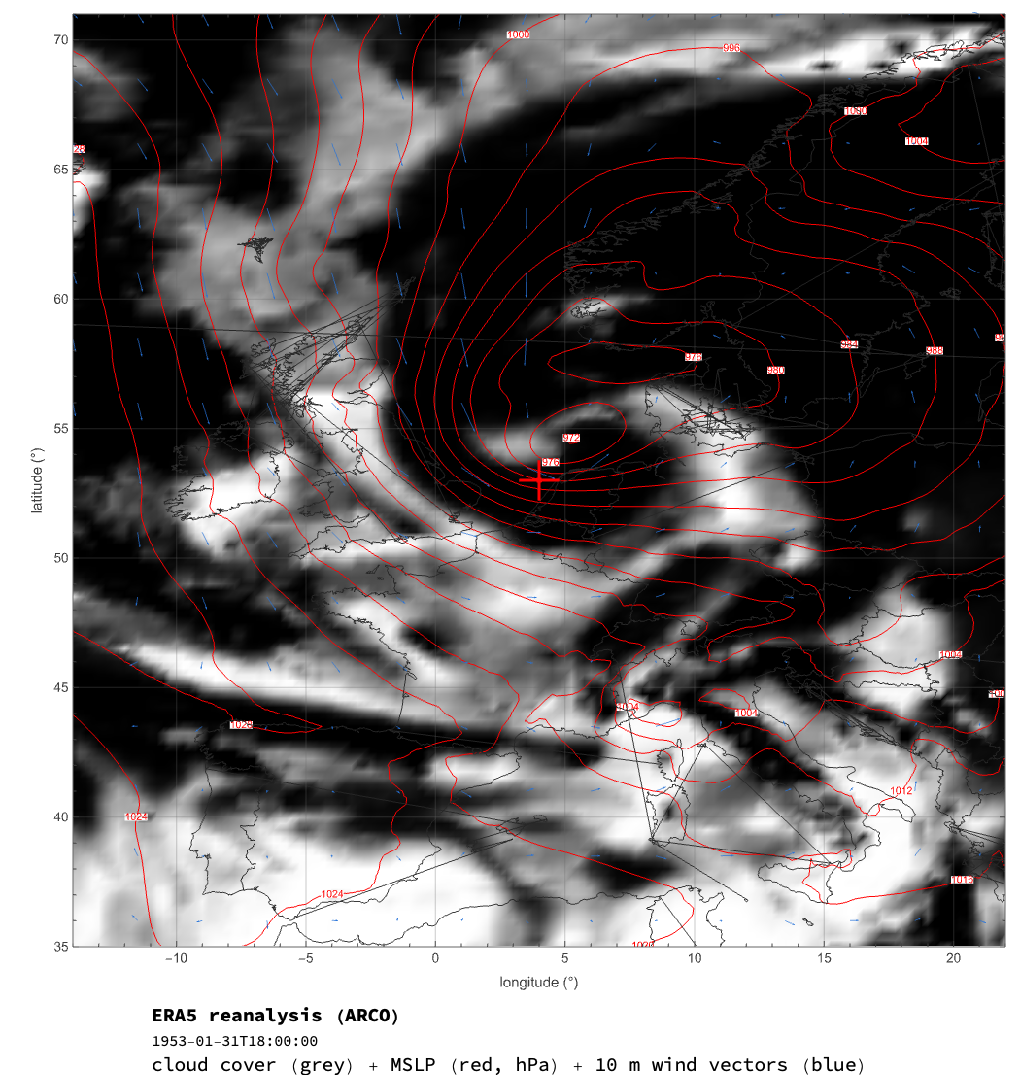
HistoricalWeatherMap produces a regional "synthetic satellite" view of the same moment. We render the cloud-cover field as a greyscale layer (white clouds, black ocean — the same convention as a thermal infrared satellite image at night), overlay mean sea-level pressure as red isobars, and add 10 m wind vectors in blue. The same call lights up an on-screen marker at the requested point.
4.4 When a real satellite is watching too
4.4 When a real satellite is watching too
For dates from 24 February 2000 onward, GIBSTrueColorImage adds a third panel: a real MODIS Terra true-colour image, served as a JPEG by NASA's GIBS WMS endpoint. Below: Hurricane Katrina on 29 August 2005, the morning of landfall. On the left, ERA5's synthetic satellite places the storm centre near MSLP 962 hPa and the wind field is unmistakeably cyclonic. On the right, the MODIS Terra orbit caught the storm at 16:35 UTC, a few hours after landfall. The eye is in the same place on both panels; the right one was photographed and the left one was reconstructed by a model that has never seen a satellite photograph.
4.5 Under the hood: one Zarr chunk per timestep
4.5 Under the hood: one Zarr chunk per timestep
Each call to HistoricalWeatherMap or HistoricalTemperatureMap resolves to two arcoBox queries (cloud + MSLP for the synthetic-satellite view, T2m + MSLP for the temperature view). Each arcoBox is one HTTPS read of a single 2 MB compressed chunk from gs://gcp-public-data-arco-era5, a ~3 s pass through the blosc / LZ4 / byte-shuffle decoder in ARCO.wl, and a lat/lon slice of the resulting 721×1440 layer. The decoded layer is cached in $arcoChunkCache keyed by {variable, timeIndex}, so subsequent same-timestamp calls (the §7 hourly animation, the §8.3 daily animation, the §5.1 event table) reuse the existing layer instead of re-fetching.
The post historically wrapped GeoDensityPlot[f, region] around Wolfram's built-in AirTemperatureData etc., which meant ~900 separate Knowledgebase round-trips per map at default resolution and several minutes per cell. Reading the ARCO chunk directly is faster, hits the full 0.25° grid without a pre-fetch step, and works back to 1 January 1940 everywhere. The Fast / GB variants are kept as aliases so older calls keep parsing, but they are no longer a distinct code path:
The post historically wrapped GeoDensityPlot[f, region] around Wolfram's built-in AirTemperatureData etc., which meant ~900 separate Knowledgebase round-trips per map at default resolution and several minutes per cell. Reading the ARCO chunk directly is faster, hits the full 0.25° grid without a pre-fetch step, and works back to 1 January 1940 everywhere. The Fast / GB variants are kept as aliases so older calls keep parsing, but they are no longer a distinct code path:
5. A walk through history
5. A walk through history
Once you have the one-liner, picking famous weather events becomes irresistible. Four storms, six decades, one dataset:
5.1 Numbers at the eye
5.1 Numbers at the eye
The interesting test for a reanalysis is whether the numbers it puts on those events agree with what was actually measured. Mean sea-level pressure is the cleanest target — there are sparse but accurate barometer readings going back centuries:
The 1987 Great Storm's central pressure is logged in independent records at roughly 953–958 hPa near the time shown; ERA5 reads 965.5 hPa at the surface point we chose, which sits a little off the centre of the storm — a 0.25° grid does not resolve the eye of a small mid-latitude cyclone to the millibar. Katrina's central pressure peaked at 902 hPa over the Gulf on 28 August and had risen to 920 hPa by the time the eyewall crossed the Louisiana coast on the morning of 29 August (NHC Tropical Cyclone Report AL122005); ERA5 reads 961.9 hPa at the chosen point an hour after landfall — an underestimate of roughly 40 hPa relative to landfall pressure, which is the expected smoothing on a 0.25° grid that cannot resolve the inner eyewall. The overall structure and timing are dead right, and the wind magnitudes (32.7 m/s, 117 km/h) are within striking distance of the maximum sustained surface winds recorded that day.
6. Interlude: the day you were born
6. Interlude: the day you were born
The ARCO ERA5 archive reaches back to 1 January 1940, which means almost everyone reading this has access to the weather of their own birthday. As a small homage to the founder of the language this post is written in, here is the sky over London at midday on Saturday 29 August 1959 — the day Stephen Wolfram was born. (We use the canonical London centroid; Interpreter["Person"]["Stephen Wolfram"]["BirthPlace"] returns the London entity itself, whose centroid lies inside the same 0.25° ERA5 grid cell as the rest of inner London.)
A settled high-pressure day in southern England: 1024 hPa, a light north-easterly off the North Sea, no rain, dry air at 54 % humidity, an afternoon overcast at 16 °C. The panel below tells the wider story: a sharp temperature contrast sits across the English Channel, with cool maritime air over the British Isles and a warm continental mass over France pushing past 22 °C.
7. Watching a hurricane come ashore
7. Watching a hurricane come ashore
A single timestamp is one cell of a four-dimensional cube; the rest of the cube is right there. Pull a list of hourly slices and you get an animation of landfall. First the static version — six three-hourly snapshots of the last 15 hours before Katrina's centre crossed the Mississippi coastline, with the minimum MSLP printed under each frame:
7.1 From frames to film
7.1 From frames to film
The strip is six frames at three-hour spacing. At hourly cadence the cube has twenty-five frames over the same window, and at that density the storm is moving smoothly enough for a real animation. In Wolfram Language the recipe is just Table + ListAnimate for an in-notebook player, or Export for a free-standing GIF / MP4:
And the result, embedded below, loops indefinitely inside the live Wolfram notebook (the PDF export below captures only the first frame — view the .nb on a Wolfram Cloud or desktop kernel for the animation):
The same one-line recipe works for any other sequence. Change the date range to follow a heatwave day by day, or scrub through a winter to watch the polar jet stream meander; swap HistoricalWeatherMap for HistoricalTemperatureMap to colour every frame by 2 m temperature; or compose two Table calls side-by-side in a GraphicsRow to compare the same atmosphere through two different fields. Because the underlying object is a 4D data cube, every "movie" is just one more slice.
7.2 After the pipeline: post-processing in Wolfram
7.2 After the pipeline: post-processing in Wolfram
The animation above is a regular WL AnimatedImage of 25 frames — which means it is also 25 Image objects waiting for Import to pick up. Wolfram's image-processing primitives can read the GIF, strip the title bar, and extract a quantitative time series from the cloud-cover field in five lines:
That gives a single number per hourly frame. Cross-referenced against the UTC clock you already know from the animation above, the result is a Wolfram-native landfall intensification curve, computed end-to-end in WL:
The post-pipeline toolkit goes a long way past MeanIntensity. Same frames, different question? ImageDifference gives you motion frame-to-frame; MorphologicalComponents segments the eyewall ring; Manipulate[frames[[i]], {i, 1, Length[frames], 1}] hands you an interactive scrubber inside any Wolfram notebook; NetModel[…] runs a convolutional classifier on the cloud field if you want to be ambitious. The animation is what carries the storm's story; the WL toolkit on top is what extracts measurements from it.
8. Computational history: the weather at Stalingrad
8. Computational history: the weather at Stalingrad
Reaching into 1942 is interesting in itself — the satellite era is still 36 years off — and it is also one of the cases where the weather is not a backdrop but a protagonist. The Wolfram knowledge graph knows about the Battle of Stalingrad as a MilitaryConflict entity; we can read its canonical start and end dates straight off, and supplement the location with the well-known coordinates of the modern city (the Knowledgebase returns Missing[NotAvailable] for "Location" on this entity at the time of writing):
Wolfram's start date (23 August 1942) corresponds to the German Luftwaffe's first major bombardment of the city itself; the broader operational battle on the Don bend approaches began on 17 July 1942, and historians use either date depending on which phase they mean. Either way: roughly six months, very nearly two million combined casualties, the longest single battle of the European war. The Soviet counter-offensive Operation Uranus opened on 19 November 1942; within four days the German Sixth Army was encircled inside an oval pocket roughly 50 km across. Manstein's relief column (Operation Winter Storm, 12–23 December) reached the Myshkova River about 48 km from the pocket's southern edge on 19–20 December; the Soviet Operation Little Saturn launched on 16 December threatened Army Group Don's northern flank, forcing Manstein to break off the relief attempt on 23 December. By mid-January the temperature inside the pocket was settling toward a record — and it was the temperature, in the end, that decided things. Paulus surrendered on 31 January 1943; the last northern resistance ended on 2 February.
8.1 The coldest hour
8.1 The coldest hour
Pulling the ERA5 temperature field over European Russia at the moment of peak cold:
8.2 Hourly temperature inside the pocket
8.2 Hourly temperature inside the pocket
Pulling the full hourly time series at the German position is also a one-liner. Below: ERA5's reading at noon, every day, from Operation Uranus to surrender. The shaded band marks sub-freezing conditions; the dashed line marks −20 °C, the temperature at which the Soviet T-34's lubricant worked normally and the German Mark III's did not.
8.3 The siege in motion
8.3 The siege in motion
And finally the cube in motion: thirty-eight two-day frames of the temperature field, looping. Watch the cold pool form over central Russia in late November, deepen and migrate south in December and early January, peak in mid-January, then collapse as Atlantic cyclones push back into the steppe in the days just before the surrender.
The point is not the spectacle. It is that "computational history" — reaching for an Entity["MilitaryConflict", …] or Entity["HistoricalEvent", …], asking it where and when a thing happened, then feeding those coordinates into a planetary reanalysis — is now small enough to fit in a paragraph of code. The same recipe will tell you the weather over D-Day beaches at 06:30 UTC on 6 June 1944, the wind that scattered the Spanish Armada (insofar as ERA5 reaches back; for 1588 you would need a different reconstruction), the heatwave under the Tour de France in July 2003, or the conditions during the road accident that took the life of someone you remember. Two centuries of weather, indexed by clock.
9. Honest caveats
9. Honest caveats
It is tempting to look at the synthetic-satellite maps and forget what they are made of.
• It is a model. Cloud cover and precipitation are diagnosed by the ECMWF Integrated Forecasting System; the reanalysis nudges that diagnosis toward observations, but the small-scale texture of a cloud field is the model's texture, not a photograph.
• Boundary-layer bias under strong inversions. Multiple validation studies (Graham et al. 2019, Batrak & Müller 2019, Albergel et al. 2018) report that ERA5's turbulence closure tends to over-mix the lowest few hundred metres on snow-covered continental surfaces and erases part of the nocturnal radiative inversion, leaving a warm bias of order 1–3 °C at 2 m — precisely the regime inside the Stalingrad anticyclone in §8. The −33.5 °C minimum the package returns is therefore likely closer to an upper bound than a lower one; the true 2 m minimum across the pocket on that morning may have been a few degrees colder. The bias direction is regime-dependent and there are publications reporting a cold bias too, so read all of these numbers with ±2–3 °C uncertainty.
• Observation density matters. Before satellite radiances entered the observation mix in 1979, ERA5 leans much more heavily on surface stations, radiosondes, ships and aircraft. For the 1953 North Sea Flood the storm track is well constrained near land, where stations were dense; over the deep Atlantic the reanalysis is doing more interpolation than fitting.
• Resolution. ERA5 lives on a 0.25° (~31 km) global grid at hourly cadence. Squall lines, tornadoes, sea breezes, and the eyewall of a small hurricane are below resolution.
• Reference frame. Temperatures are at 2 m above the model's own elevation surface, not the station thermometer reading you would read in a record book; over rough terrain the two can differ by several degrees.
• The numbers are still extraordinary. ERA5 places Katrina's track and timing essentially correctly (while underestimating the eyewall central pressure by ≈40 hPa, as discussed in §5.1), puts the 1987 Great Storm exactly where it was, and pins the 2003 heatwave to the right week. It is the best four-dimensional record of the recent atmosphere that exists — and the Wolfram Language is one DateObject away from it.
• Boundary-layer bias under strong inversions. Multiple validation studies (Graham et al. 2019, Batrak & Müller 2019, Albergel et al. 2018) report that ERA5's turbulence closure tends to over-mix the lowest few hundred metres on snow-covered continental surfaces and erases part of the nocturnal radiative inversion, leaving a warm bias of order 1–3 °C at 2 m — precisely the regime inside the Stalingrad anticyclone in §8. The −33.5 °C minimum the package returns is therefore likely closer to an upper bound than a lower one; the true 2 m minimum across the pocket on that morning may have been a few degrees colder. The bias direction is regime-dependent and there are publications reporting a cold bias too, so read all of these numbers with ±2–3 °C uncertainty.
• Observation density matters. Before satellite radiances entered the observation mix in 1979, ERA5 leans much more heavily on surface stations, radiosondes, ships and aircraft. For the 1953 North Sea Flood the storm track is well constrained near land, where stations were dense; over the deep Atlantic the reanalysis is doing more interpolation than fitting.
• Resolution. ERA5 lives on a 0.25° (~31 km) global grid at hourly cadence. Squall lines, tornadoes, sea breezes, and the eyewall of a small hurricane are below resolution.
• Reference frame. Temperatures are at 2 m above the model's own elevation surface, not the station thermometer reading you would read in a record book; over rough terrain the two can differ by several degrees.
• The numbers are still extraordinary. ERA5 places Katrina's track and timing essentially correctly (while underestimating the eyewall central pressure by ≈40 hPa, as discussed in §5.1), puts the 1987 Great Storm exactly where it was, and pins the 2003 heatwave to the right week. It is the best four-dimensional record of the recent atmosphere that exists — and the Wolfram Language is one DateObject away from it.
10. How the package reaches ARCO ERA5 from pure Wolfram
10. How the package reaches ARCO ERA5 from pure Wolfram
Every map and every point reading in this post comes from the ARCO ERA5 store on Google Cloud (gs://gcp-public-data-arco-era5, anonymous, no API key). The store is a Zarr v2 group — each variable is a 3D array of shape {1323648, 721, 1440} (hours since 1900, latitudes 90−90, longitudes 0359.75), chunked one timestep at a time and compressed with blosc1 + LZ4 + byte shuffle. The companion ARCO.wl file is a pure-Wolfram reader for that wire format: ~200 lines of WL covering the LZ4 raw-block decompressor, the blosc1 wrapper, the inverse byte-shuffle filter and a small HTTPS + cache layer. Assuming the package has already been loaded by an earlier cell, fetching the landfall-hour cloud cover at the Katrina grid point is one Wolfram cell:
The reader caches every decoded chunk for the session, so subsequent same-timestamp lookups are instant; the first call to a new timestamp is dominated by the ~2 MB HTTP download and a ~3 s blosc/LZ4 decode pass. Every ERA5 surface variable the package needs — 2m_temperature, 2m_dewpoint_temperature, mean_sea_level_pressure, 10m_u_component_of_wind, 10m_v_component_of_wind, total_precipitation, total_cloud_cover — travels through this single decoder. Every pressure-level and model-level field in ARCO ERA5 uses the same chunk format, so the reader generalises to anything else in the store by changing the variable name. arcoBox returns a labelled box of values around a centre point and half-width (the maps in §4 – §8 are built from this primitive); arcoChunkLayer returns a full 721×1440 timestep layer if you want to slice it yourself. The chunk cache is keyed by {variable, timeIndex} so a 25-frame Katrina animation pulls each unique cell exactly once — subsequent same-timestamp requests inside a session return immediately.
A parallel route into climate data from inside Wolfram, also worth knowing about, is Diego Zviovich's recent Google Earth Engine paclet for climate and weather analysis on the Wolfram Community; that paclet authenticates through GEE and exposes the full GEE catalogue (Landsat, MODIS, ECMWF reanalyses, high-resolution land-cover and so on), where the package described here goes directly to one specific Zarr store with no auth. The two approaches are complementary.
A parallel route into climate data from inside Wolfram, also worth knowing about, is Diego Zviovich's recent Google Earth Engine paclet for climate and weather analysis on the Wolfram Community; that paclet authenticates through GEE and exposes the full GEE catalogue (Landsat, MODIS, ECMWF reanalyses, high-resolution land-cover and so on), where the package described here goes directly to one specific Zarr store with no auth. The two approaches are complementary.
11. Acknowledgements & data attribution
11. Acknowledgements & data attribution
The source code attached to this post is released under the MIT licence (the licence header is at the top of the HistoricalWeather.wl attachment). The data and imagery the code fetches at runtime are governed by the licences of their providers, which must be reproduced when this work is published or reused:
• ERA5 (every cloud-cover, temperature, pressure and wind field in this post, whether reached directly via the ARCO Zarr store or indirectly via Wolfram's AirTemperatureData family) is produced by ECMWF and distributed by the Copernicus Climate Change Service (C3S) under the Licence to Use Copernicus Products. When publishing derived figures, please:
1. add the acknowledgement "Generated using Copernicus Climate Change Service information [year of access]";
2. cite Hersbach, H. et al. (2020), "The ERA5 global reanalysis", QJRMS 146(730), 1999–2049, doi:10.1002/qj.3803;
3. include the standard disclaimer: "Neither the European Commission nor ECMWF is responsible for any use that may be made of the Copernicus information or data this product contains."
• MODIS Terra true-colour imagery (the right panel of Figure 4, and anything returned by GIBSTrueColorImage) is provided by NASA's Global Imagery Browse Services (GIBS), part of NASA's Earth Science Data and Information System (ESDIS). NASA asks publications to add the acknowledgement "We acknowledge the use of imagery provided by services from NASA's Global Imagery Browse Services (GIBS), part of NASA's Earth Science Data and Information System (ESDIS)."
• Battle of Stalingrad metadata (dates, location, casualty count in §8) is supplied by the Wolfram Knowledgebase via Entity["MilitaryConflict", "BattleOfStalingrad"]. Wolfram knowledge entries remain the property of Wolfram Research and their use is governed by your Wolfram Engine / Mathematica / Wolfram Cloud licence.
• Country borders and coastlines overlaid on the regional maps come from GeoBoundary of the relevant Entity["Country", …] records in the Wolfram Knowledgebase.
• Stephen Wolfram's date and place of birth in §6 are public-domain biographical facts; they are also surfaced by the Wolfram Knowledgebase itself — for instance Interpreter["Person"]["Stephen Wolfram"]["BirthDate"] returns DateObject[{1959, 8, 29}] and the corresponding "BirthPlace" property returns the London entity — so the same biographical lookup is itself a one-liner in the language this post is written in.
1. add the acknowledgement "Generated using Copernicus Climate Change Service information [year of access]";
2. cite Hersbach, H. et al. (2020), "The ERA5 global reanalysis", QJRMS 146(730), 1999–2049, doi:10.1002/qj.3803;
3. include the standard disclaimer: "Neither the European Commission nor ECMWF is responsible for any use that may be made of the Copernicus information or data this product contains."
• MODIS Terra true-colour imagery (the right panel of Figure 4, and anything returned by GIBSTrueColorImage) is provided by NASA's Global Imagery Browse Services (GIBS), part of NASA's Earth Science Data and Information System (ESDIS). NASA asks publications to add the acknowledgement "We acknowledge the use of imagery provided by services from NASA's Global Imagery Browse Services (GIBS), part of NASA's Earth Science Data and Information System (ESDIS)."
• Battle of Stalingrad metadata (dates, location, casualty count in §8) is supplied by the Wolfram Knowledgebase via Entity["MilitaryConflict", "BattleOfStalingrad"]. Wolfram knowledge entries remain the property of Wolfram Research and their use is governed by your Wolfram Engine / Mathematica / Wolfram Cloud licence.
• Country borders and coastlines overlaid on the regional maps come from GeoBoundary of the relevant Entity["Country", …] records in the Wolfram Knowledgebase.
• Stephen Wolfram's date and place of birth in §6 are public-domain biographical facts; they are also surfaced by the Wolfram Knowledgebase itself — for instance Interpreter["Person"]["Stephen Wolfram"]["BirthDate"] returns DateObject[{1959, 8, 29}] and the corresponding "BirthPlace" property returns the London entity — so the same biographical lookup is itself a one-liner in the language this post is written in.
Thanks to Diego Zviovich for his recent Wolfram Community post on the Google Earth Engine paclet for climate and weather analysis, which appeared while I was preparing this post. It comes at the same problem — climate data into Wolfram in one cell — from the opposite direction: a thin WL gateway to the full GEE catalogue, where ARCO.wl here reads one specific ECMWF Zarr store directly. Two complementary routes.
12. References & links
12. References & links
• H. Hersbach et al., "The ERA5 global reanalysis", Quarterly Journal of the Royal Meteorological Society 146(730), 1999–2049 (2020). doi:10.1002/qj.3803.
• Copernicus Weather Replay app — weather-replay.climate.copernicus.eu.
• ARCO-ERA5 Zarr store on Google Cloud — github.com/google-research/arco-era5.
• NASA Global Imagery Browse Services (GIBS) — gibs.earthdata.nasa.gov.
• Source code — the Wolfram package used throughout this post is attached to the post as HistoricalWeather.wl, MIT-licensed.
• Related Wolfram Community work — Diego Zviovich, "Google Earth Engine (GEE) paclet: Climate and Weather Analysis", a complementary WL gateway into Google's geospatial-data catalogue (the present post reaches the ARCO ERA5 Zarr store directly; Zviovich's paclet authenticates through Google Earth Engine and exposes Landsat, MODIS, ECMWF and many other datasets through the GEE REST API). Two routes into climate data from a single Wolfram notebook.
• Copernicus Weather Replay app — weather-replay.climate.copernicus.eu.
• ARCO-ERA5 Zarr store on Google Cloud — github.com/google-research/arco-era5.
• NASA Global Imagery Browse Services (GIBS) — gibs.earthdata.nasa.gov.
• Source code — the Wolfram package used throughout this post is attached to the post as HistoricalWeather.wl, MIT-licensed.
• Related Wolfram Community work — Diego Zviovich, "Google Earth Engine (GEE) paclet: Climate and Weather Analysis", a complementary WL gateway into Google's geospatial-data catalogue (the present post reaches the ARCO ERA5 Zarr store directly; Zviovich's paclet authenticates through Google Earth Engine and exposes Landsat, MODIS, ECMWF and many other datasets through the GEE REST API). Two routes into climate data from a single Wolfram notebook.
CITE THIS NOTEBOOK
CITE THIS NOTEBOOK
Time travel through the Atmosphere: replaying historical weather from 1940 to today
by Marco Thiel
Wolfram Community, STAFF PICKS, May 18, 2026
https://community.wolfram.com/groups/-/m/t/3717198
by Marco Thiel
Wolfram Community, STAFF PICKS, May 18, 2026
https://community.wolfram.com/groups/-/m/t/3717198