This is collaborative work by Tobias Ahsendorf, Felix Wong, Roland Eils & Jeremy Gunawardena
ABSTRACT (original article): Gene regulation has, for the most part, been quantitatively analysed by assuming that regulatory mechanisms operate at thermodynamic equilibrium. This formalism was originally developed to analyse the binding and unbinding of transcription factors from naked DNA in eubacteria. Although widely used, it has made it difficult to understand the role of energy-dissipating, epigenetic mechanisms, such as DNA methylation, nucleosome remodelling and post-translational modification of histones and co-regulators, which act together with transcription factors to regulate gene expression in eukaryotes.
Results
Here, we introduce a graph-based framework that can accommodate non-equilibrium mechanisms. A gene-regulatory system is described as a graph, which specifies the DNA microstates (vertices), the transitions between microstates (edges) and the transition rates (edge labels). The graph yields a stochastic master equation for how microstate probabilities change over time. We show that this framework has broad scope by providing new insights into three very different ad hoc models, of steroid-hormone responsive genes, of inherently bounded chromatin domains and of the yeast PHO5 gene. We find, moreover, surprising complexity in the regulation of PHO5, which has not yet been experimentally explored, and we show that this complexity is an inherent feature of being away from equilibrium. At equilibrium, microstate probabilities do not depend on how a microstate is reached but, away from equilibrium, each path to a microstate can contribute to its steady-state probability. Systems that are far from equilibrium thereby become dependent on history and the resulting complexity is a fundamental challenge. To begin addressing this, we introduce a graph-based concept of independence, which can be applied to sub-systems that are far from equilibrium, and prove that history-dependent complexity can be circumvented when sub-systems operate independently.
Conclusions
As epigenomic data become increasingly available, we anticipate that gene function will come to be represented by graphs, as gene structure has been represented by sequences, and that the methods introduced here will provide a broader foundation for understanding how genes work.
CITATION (original article): Ahsendorf, T., Wong, F., Eils, R. et al. A framework for modelling gene regulation which accommodates non-equilibrium mechanisms. BMC Biol 12, 102 (2014). https://doi.org/10.1186/s12915-014-0102-4
Introduction
Introduction
We started by developing a mathematical way to understand how genes are controlled. I began with a simple bacterium called *E. coli*, where we looked at how proteins called transcription factors stick to and unstick from DNA. We assumed these processes happened very quickly and reached a stable balance. Using physics principles, I could then calculate which DNA patterns were most likely and predict how fast genes would be turned on or off based on the amounts of different proteins present.
This method worked well for bacteria. However, we then moved to more complex organisms like yeast, flies, and humans. Here, we ran into a problem. These organisms use energy-consuming processes to reorganize their DNA and modify proteins in ways that bacteria don’t. Despite knowing that energy is being used to drive these systems away from natural balance, we still applied our old method anyway. Some experiments suggested this wasn’t quite right, especially for how DNA wraps around proteins called nucleosomes.
A scientist named John Hopfield explained why this matters: if a system sits at perfect balance, there’s a hard limit to how accurate it can be at copying or processing information. To do better, we must expend energy. He showed that by spending energy cleverly, cells could make nearly perfect copies and detect errors perfectly. Yet despite understanding this, we still weren’t sure how important energy-spending really is for controlling genes in complex organisms.
The main barrier was that nobody had a good mathematical toolkit to handle these energy-spending processes. We developed a new framework based on graphs and connections that doesn’t require systems to be at balance. The framework views genes in terms of reactions and rates rather than just energies and states. If a system is perfectly balanced, our framework simplifies back to the old method, confirming it still works for simpler cases.
We have three main goals here. First, we introduce this new framework and show it works for three different gene regulation problems. Second, we demonstrate that one particular gene in yeast shows surprisingly complex behavior that we can explain as a natural feature of energy-spending systems. Third, we explore when this complexity simplifies and becomes easier to predict. To make this accessible, we start with intuitive explanations before diving into the mathematical details.
Constructing polynomials generated by the Matrix-Tree Theorem
Constructing polynomials generated by the Matrix-Tree Theorem
This section is for constructing and manipulating polynomials generated by the Matrix-Tree Theorem, as applied to the Laplacian matrix of a labelled, directed graph.
Background
Background
The linear framework is based on a labelled, directed graph, G, which gives rise to a dynamics, x/t = ℒ(G).x, where ℒ(G) is the Laplacian matrix of G [1]. This linear dynamics can be thought of as as first-order chemistry or as the corresponding stochastic master equation [2] and has wide applications in different biological contexts [3,4]. The steady-states of this dynamics or, equivalently, the elements of the kernel of the Laplacian, are the subject of interest. For a strongly-connected graph, the kernel of the Laplacian has dimension 1 and a basis element can be constructed by the Matrix-Tree Theorem [1].
This notebook provides capabilities for the linear framework, which is developed in a series of papers [1,2,3,4].
Usage
Usage
Before using this notebook, a text file with the extension .txt should be created (for example, graph.txt) in which a graph is described as a list of triples, (i,a,j), signifying a directed edge from vertex i to vertex j with label a. The graph is assumed to be strongly connected. The python script MTT.py (see Further Information below) should then be executed. This reads graph.txt and produces, for each vertex i in the graph, a file graph-i.txt, which enumerates the spanning trees rooted at i, as prescribed by the Matrix-Tree Theorem. The script also produces a cleaned description of the graph in the file graph-parsed.txt. This notebook reads these files and expects to be executed in the directory which contains them.
Set the variable name GraphName below to the name of the graph in the graph description file (ie: GraphName = “graph” if the file is graph.txt) and then execute the functions below. The notebook builds the basis vector ρ (called here “rho”) in the kernel of the Laplacian matrix of the graph. For each vertex i, the i-th component of the basis vector is created as a polynomial in the edge labels
rhoi[,...,]
a
1
a
n
with the labels ordered as they appear in graph.txt.These polynomials can then be interrogated using Mathematica functions, as required, depending on the context.
Method details
Method details
The script MTT.py and further details, including contact information, are available at https://vcp.upf.edu/software.html#linear. This notebook was developed by Felix Wong for the paper [4].
Instructional method
Instructional method
Kim-O’Shea model for the yeast PHO5 gene
Kim-O’Shea model for the yeast PHO5 gene
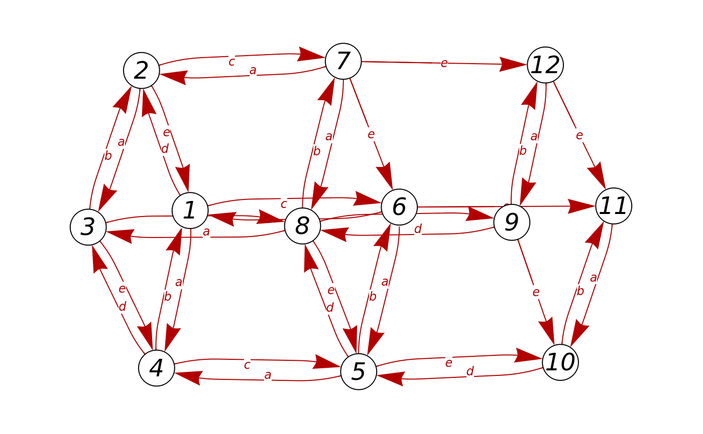
This section is specialised to the graph of the Kim-O’Shea model for the yeast PHO5 gene. For this strongly connected graph, the code reads files listing the spanning trees rooted at each vertex. Using these trees, it constructs the entries of the steady-state basis vector, ρ (rho), as polynomials in the edge labels.
This detailed calculation confirmed the significant complexity inherent in the PHO5 gene regulation model, illustrating the principle that non-equilibrium systems depend fundamentally on “history,” requiring the summation over every spanning tree (or path) to determine the steady-state probability
Starting on a fresh kernel
Quit[]
We specify Kimoshea graph
GraphName="kimoshea";graph=Import[NotebookDirectory[]<>GraphName<>"-parsed.txt","Table"];MathematicaGraph=ToExpression[StringReplace[ToString[graph],{"{{""{","}}""}","(""{",")""}","'""\""}]]/.{f_Integer,m_,l_Integer}{fl,ToString[m]};(*getlabels*)listoflabels=DeleteDuplicates[MathematicaGraph[[All,2]]];lstring="{";For[m=1,m≤Length[listoflabels],m++,lstring=lstring<>"{"<>ToString[m]<>",\""<>listoflabels[[m]]<>"\"},";]flstring=StringDrop[lstring,-1]<>"}";ToExpression["labelrule="<>flstring];(*functionthatcomesinhandywhenplotting*)HashString[f_String]:=Mean[ToCharacterCode[f]]+ToCharacterCode[f].ToCharacterCode[f]
Plotting the graph in 2D and 3D
GraphPlotMathematicaGraph,
In 3D
GraphPlot3DMathematicaGraph,

Make the components of the basis vector rho, in the kernel of the Laplacian
Initializing variables and functions
Find number of nodes in graph
Find number of nodes in graph
numberofnodes=Max[MathematicaGraph/.{f_Integer->l_Integer,m_String}{f,l}];rhofnarg="";identityelement="";For[m=1,m≤Length[listoflabels],m++,rhofnarg=rhofnarg<>labelrule[[m]][[2]]<>"_,";identityelement=identityelement<>"1,";]rhoargument=StringDrop[rhofnarg,-1];identity=StringDrop[identityelement,-1];
Build the rho’ s from the imported data
Work out the total number of spanning trees in the graph
Number of spanning trees is sum of rho_i’ s at identity
Print out the rhoi. Note that rhotot gives rho1 + ... + rhon (ie: the partition function)
Construct the numerator of the Pho5 gene regulation function (see the paper) and count the number of monomials
The denominator of the gene regulation function is given by the partition function
Fitting to the experimental data for PHO5 promoter variants
Fitting to the experimental data for PHO5 promoter variants
This section shows how the calculated PHO5 gene regulation function discussed in the section on “History-dependent complexity away from equilbrium” can be fitted to experimental data from the paper by Kim & O’Shea cited in [5] below.
Kim & O’Shea provide data for several promoter variants, of which we consider the variants LL, LH, HH, HL, LX, HX, where L means “low affinity”, H means “high affinity” and X means “deleted” (for further details, see [5]). The wild-type corresponds to variant LH, as described in Paper Figure 7. Each variant gives rise to a different graph, which use the same labels as in the wild-type graph. The variants LX and HX give rise to a 8-vertex graph, which has the same unlabelled structure in both cases. The remaining variants, LL, LH, HH, HL, give rise to the same unlabelled 12-vertex graph as in the wild-type. The two graphs are shown below, the one on the right corresponding to the wild-type graph in Paper Figure 7B.
Kim & O’Shea provide data for several promoter variants, of which we consider the variants LL, LH, HH, HL, LX, HX, where L means “low affinity”, H means “high affinity” and X means “deleted” (for further details, see [5]). The wild-type corresponds to variant LH, as described in Paper Figure 7. Each variant gives rise to a different graph, which use the same labels as in the wild-type graph. The variants LX and HX give rise to a 8-vertex graph, which has the same unlabelled structure in both cases. The remaining variants, LL, LH, HH, HL, give rise to the same unlabelled 12-vertex graph as in the wild-type. The two graphs are shown below, the one on the right corresponding to the wild-type graph in Paper Figure 7B.
Usage
Usage
Ensure that the accompanying Mathematica packages GRFs.m and KimOSheaData.m are in the same directory and then execute the notebook.
Further information
Further information
The package containing this notebook, along with the accompanying files, is available from our website at https://vcp.upf.edu/software.html#linear, as a gzipped tar archive. The website also provides further background about the linear framework, on which these calculations are based, and further contact information.This notebook was developed by Felix Wong for the paper [4].
Starting on a fresh kernel
Import accompanying packages
Font used in the plots of this section
Normalise the YFP and CFP values
Normalise the YFP and CFP values
Normalise the YFP and CFP values by the corresponding RFP value plot the experimental data for each promoter variant.
Create data structure for each variant
Plot options for first 3 plots
Show plots
Smoothing the data
Smoothing the data
Smooth the data by taking a moving average of 15 nearest-neighbor data points and plot by variant.
Compute moving average for each variant
Plot smoothed data
As a sanity check, display a moving average plot of just the variants LH and HL, which should resemble a smoothed version of the plot in Figure 2 of the Kim & O’Shea paper.
Calculating the GRF and making a collective fit to all variants simultaneously
Calculating the GRF and making a collective fit to all variants simultaneously
The concentration of Pho4, [Pho4], is assumed to be proportional to nYFP (normalised YFP). The constant of proportionality is not known but it can be absorbed into the parameter K in the Hill function. Accordingly, we assumed that the input to the GRF was given by nYFP. Since the output of the GRF is the probability of transcription, we scaled the experimental data to its maximum expression level. An additional scale factor could be introduce for each variant if necessary but this adds to the complexity without conveying any more information, so we chose not to do that here.
We de-dimensionalised the rate constants in the graph,
These are represented by the variables a, b, c, d, and e, respectively, in the calculations below. In this way, the total number of parameters is five, given by one dimensional quantity and four non-dimensional quantities,
Next, we plot all six variants, showing for each the calculated GRF overlayed on the corresponding experimental data, using the same five parameter values, which can be manipulated collectively across all six variants. In this way, a collective fit to all the data can be manually found. The following numerical values for the five parameters give a reasonable qualitative fit
Concatenate GRF functions depending on variant
Plot options for following plot
Create normalized plots
Show plots
Individual plots for each variant
Individual plots for each variant
Plot options for following
Show plot - by - plot
Fits of the data to each individual variant using Levenberg-Marquardt
Fits of the data to each individual variant using Levenberg-Marquardt
Show plot - by - plot
References
References
[1] J. Gunawardena, “A linear framework for time-scale separation in nonlinear biochemical systems”, PLoS ONE 7:e36321, 2012. https://doi.org/10.1371/journal.pone.0036321
[2] Mirzaev, I., Gunawardena, J. Laplacian Dynamics on General Graphs. Bull Math Biol 75, 2118–2149 (2013). https://doi.org/10.1007/s11538-013-9884-8
[3] J. Gunawardena, “Time-scale separation: Michaelis and Menten’s old idea, still bearing fruit”, FEBS J, invited review, in press, 2013. https://doi.org/10.1111/febs.12532
[4] Ahsendorf, T., Wong, F., Eils, R. et al. A framework for modelling gene regulation which accommodates non-equilibrium mechanisms. BMC Biol 12, 102 (2014). https://doi.org/10.1186/s12915-014-0102-4
[5] Kim, H., O’Shea, E. A quantitative model of transcription factor–activated gene expression. Nat Struct Mol Biol 15, 1192–1198 (2008). https://doi.org/10.1038/nsmb.1500
CITE THIS NOTEBOOK
CITE THIS NOTEBOOK
A framework for modelling gene regulation which accommodates non-equilibrium mechanisms
by Tobias Ahsendorf, Felix Wong, Roland Eils & Jeremy Gunawardena
Wolfram Community, STAFF PICKS, November 26, 2025
https://community.wolfram.com/groups/-/m/t/3582366
by Tobias Ahsendorf, Felix Wong, Roland Eils & Jeremy Gunawardena
Wolfram Community, STAFF PICKS, November 26, 2025
https://community.wolfram.com/groups/-/m/t/3582366