Endogeneity Bias

parameters of true linear model

0.5

correlation between independent variable and error term

-0.76

true model

true model points

observed data points

OLS estimation

generate data

parameters of distributions

Endogeneity is one of the major concerns of contemporary empirical studies in economics and econometrics. This Demonstration aims to show the geometric sense of this phenomenon in the simplest setting, namely the model with one single explanatory variable (also known as the independent variable).

We use a population regression function[1] of the simple form

Y=α+βX

, where

and

are true parameters that are never known, to generate observable data of the form

=α+β

, where

is the error term (or disturbance) for each simulated observation

. Simulated variation of the error term is controlled by the parameter

. The purpose of fitting methods such as ordinary least squares (OLS) is to estimate true parameters of the model given observable data. A fitted model usually has the form



=a+bX

(sample regression function[1]).

The parameter

is most important for this Demonstration. It is used to model the correlation between the vectors

and

, that is, if

ρ=0

, then there is no covariance between the vectors; otherwise there is covariance that is maximal at

ρ=1

(or

ρ=-1

Details

Endogeneity bias (in the narrow sense) is applicable to the model if

cov(X,ϵ)≠0

. Whenever

cov(X,ϵ)=0

(meaning that the independent variable

is not correlated with the error term

), there is no endogeneity bias (in the narrow sense). In this case, the slope of the fitting curve (OLS regression line) converges to the slope of the true line

with the growth of the number of observations

, or

lim

n∞

b(n)=β

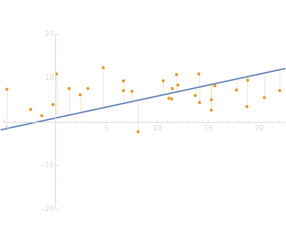
On the contrary, with endogeneity bias there is no such convergence and the fitting model gives inconsistent estimates of

in terms of

. You can also see a geometric representation of endogeneity in that simple case when observations (points on the plot) lie systematically lower or higher than a given true line. That is what makes OLS fitting pointless in the presence of endogeneity bias. There are many reasons of endogeneity, namely, omitted variables, measurement errors, and simultaneity. Methods such as using a control function or instrumental variables (IV) can be applied to cure the endogeneity bias problem.

This Demonstration is designed to generate random data by clicking the "generate data" button. You can vary the parameters:

is the number of observations,

is both (for simplicity of the model) the expectation and the standard error of the random variate

, and

is the standard error of the normally distributed error term

with

expectation.

References

[1] J. M. Wooldridge, Introductory Econometrics: A Modern Approach, Mason, OH: South-Western, Cengage Learning, 2009 p. 26.

Permanent Citation

Timur Gareev

"Endogeneity Bias"
http://demonstrations.wolfram.com/EndogeneityBias/
Wolfram Demonstrations Project
Published: February 8, 2016