Conchoids::usage="Reference:WolframMathWorld:Conchoid;ConchoidofdeSluzePersonal.;";
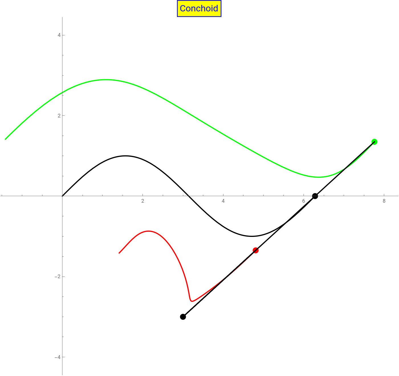
Example 1: Sine’s conchoid
In[]:=
SwatchLegend[{Green,Red,Black},{"Positive Conchoid","Negative Conchoid","Original function"}]Manipulatef[t_]:=t;g[t_]:=Sin[t];=3;=-3;k=2;[t_]:=f[t]++,g[t]++;[t_]:=f[t]-+,g[t]-+;Show{ParametricPlot[[t],{t,0,t1},PlotStyle{Green,Thick},PerformanceGoal->"Quality"],ParametricPlot[[t],{t,0,t1},PlotStyle{Red,Thick},PerformanceGoal->"Quality"],ParametricPlot[{f[t],g[t]},{t,0,2π},PlotStyle{Black,Thick}],Graphics[{Green,PointSize[0.015],Point[[t1]]}],Graphics[{Red,PointSize[0.015],Point[[t1]]}],Graphics[{Black,Thick,Line[{[t1],{,},[t1]}]}],Graphics[{Black,PointSize[0.015],Point[{,}]}],Graphics[{Black,PointSize[0.015],Point[{f[t1],g[t1]}]}]},AxesTrue,AxesOrigin{0,0},AspectRatioAutomatic,ImageSize700,PlotRange-,2.5π,{-4,4},PlotLabelStyle[Framed["Conchoid"],16,Blue,BackgroundYellow],{{t1,0.00002,"Value (t1)"},0.00001,2π,0.00001},ControlPlacement->Top
x
0
y
0
ζ
+
k(f[t]-)
x
0
2
(f[t]-)
x
0
2
(g[t]-)
y
0
k(g[t]-)
y
0
2
(f[t]-)
x
0
2
(g[t]-)
y
0
ζ
-
k(f[t]-)
x
0
2
(f[t]-)
x
0
2
(g[t]-)
y
0
k(g[t]-)
y
0
2
(f[t]-)
x
0
2
(g[t]-)
y
0
ζ
+
ζ
-
ζ
+
ζ
-
ζ
-
x
0
y
0
ζ
+
x
0
y
0
π
3
Out[]=


Out[]=


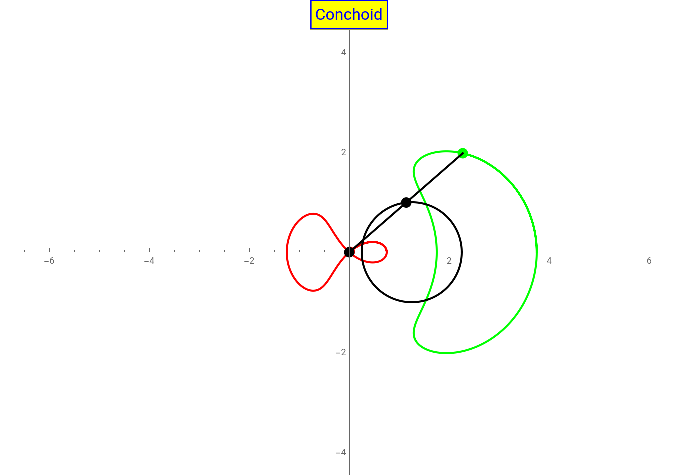
Example 2: Circle’s conchoid
In[]:=
SwatchLegend[{Green,Red,Black},{"Positive Conchoid","Negative Conchoid","Original function"}]Manipulatef[t_]:=Cos[t]+1.25;g[t_]:=Sin[t];=0;=0;k=1.5;[t_]:=f[t]++,g[t]++;[t_]:=f[t]-+,g[t]-+;Show[{ParametricPlot[[t],{t,-2π,t1},PlotStyle{Green,Thick},PerformanceGoal->"Quality"],ParametricPlot[[t],{t,-2π,t1},PlotStyle{Red,Thick},PerformanceGoal->"Quality"],ParametricPlot[{f[t],g[t]},{t,0,2π},PlotStyle{Black,Thick}],Graphics[{Green,PointSize[0.015],Point[[t1]]}],Graphics[{Red,PointSize[0.015],Point[[t1]]}],Graphics[{Black,Thick,Line[{[t1],{,},[t1]}]}],Graphics[{Black,PointSize[0.015],Point[{,}]}],Graphics[{Black,PointSize[0.015],Point[{f[t1],g[t1]}]}]},AxesTrue,AxesOrigin{0,0},AspectRatioAutomatic,ImageSize700,PlotRange{{-2π,2π},{-4,4}},PlotLabelStyle[Framed["Conchoid"],16,Blue,BackgroundYellow]],{{t1,-2π+0.00002,"Value (t1)"},-2π+0.00001,2π,0.00001},ControlPlacement->Top
x
0
y
0
ζ
+
k(f[t]-)
x
0
2
(f[t]-)
x
0
2
(g[t]-)
y
0
k(g[t]-)
y
0
2
(f[t]-)
x
0
2
(g[t]-)
y
0
ζ
-
k(f[t]-)
x
0
2
(f[t]-)
x
0
2
(g[t]-)
y
0
k(g[t]-)
y
0
2
(f[t]-)
x
0
2
(g[t]-)
y
0
ζ
+
ζ
-
ζ
+
ζ
-
ζ
-
x
0
y
0
ζ
+
x
0
y
0
Out[]=
Out[]=
Example 3: Ellipse’s conchoid
In[]:=
SwatchLegend[{Green,Red,Black},{"Positive Conchoid","Negative Conchoid","Original function"}]Manipulatef[t_]:=3Cos[t];g[t_]:=2Sin[t];=0;=1.5;k=1.5;[t_]:=f[t]++,g[t]++;[t_]:=f[t]-+,g[t]-+;Show[{ParametricPlot[[t],{t,0,t1},PlotStyle{Green,Thick},PerformanceGoal->"Quality"],ParametricPlot[[t],{t,0,t1},PlotStyle{Red,Thick},PerformanceGoal->"Quality"],ParametricPlot[{f[t],g[t]},{t,0,2π},PlotStyle{Black,Thick}],Graphics[{Green,PointSize[0.015],Point[[t1]]}],Graphics[{Red,PointSize[0.015],Point[[t1]]}],Graphics[{Black,Thick,Line[{[t1],{,},[t1]}]}],Graphics[{Black,PointSize[0.015],Point[{,}]}],Graphics[{Black,PointSize[0.015],Point[{f[t1],g[t1]}]}]},AxesTrue,AxesOrigin{0,0},AspectRatioAutomatic,ImageSize700,PlotRange{{-2π,2π},{-4,5}},PlotLabelStyle[Framed["Conchoid"],16,Blue,BackgroundYellow]],{{t1,0.00002,"Value (t1)"},0.00001,2π,0.00001},ControlPlacement->Top
x
0
y
0
ζ
+
k(f[t]-)
x
0
2
(f[t]-)
x
0
2
(g[t]-)
y
0
k(g[t]-)
y
0
2
(f[t]-)
x
0
2
(g[t]-)
y
0
ζ
-
k(f[t]-)
x
0
2
(f[t]-)
x
0
2
(g[t]-)
y
0
k(g[t]-)
y
0
2
(f[t]-)
x
0
2
(g[t]-)
y
0
ζ
+
ζ
-
ζ
+
ζ
-
ζ
-
x
0
y
0
ζ
+
x
0
y
0
Example 4: Nicomedes conchoid