Time Evolution of the Wavefunction in a 1D Infinite Square Well
Time Evolution of the Wavefunction in a 1D Infinite Square Well


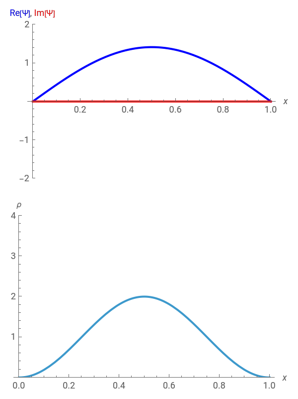
This Demonstration shows some solutions to the time-dependent Schrödinger equation for a 1D infinite square well. You can see how wavefunctions and probability densities evolve in time. You can set initial conditions as a linear combination of the first three energy eigenstates.
Details
Details
Vary the time to see the evolution of the wavefunction of a particle of mass in an infinite square well of length . Initial conditions are a linear combination of the first three energy eigenstates . The amplitude of each coefficient is set by the sliders. The phase of each coefficient at is set by the sliders. The wavefunction is automatically normalized.
t
m
L
ψ
n
a
t=0
p
Position is in units of .
L
Ψ
-1/2
L
ρ
-1
L
Energy is in units of /2.
2
ℏ
2
π
2
mL
Time is in units of energy units).
ℏ/(2π
External Links
External Links
Permanent Citation
Permanent Citation
Jonathan Weinstein, (University of Nevada, Reno)
"Time Evolution of the Wavefunction in a 1D Infinite Square Well"
http://demonstrations.wolfram.com/TimeEvolutionOfTheWavefunctionInA1DInfiniteSquareWell/
Wolfram Demonstrations Project
Published: June 13, 2011