Strong Acid – Strong Base Titration Using Arc-Length Continuation
Authors: Housam Binous
Strong Acid – Strong Base Titration Using Arc-Length Continuation
Authors: Housam Binous
Authors: Housam Binous
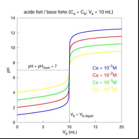
We reproduce the classical strong acid / strong base titration curve shown in the figure below:However, instead of directly plotting the analytical formula, the solution branch is traced numerically using an arc-length continuation method.The continuation algorithm steps are as follows:1- Defines the nonlinear equilibrium equation.2- Computes a tangent vector.3- Performs a predictor step.4- Applies a Newton corrector.5- Continues along the pH curve through the steep equivalence region.References: [1] https://ressources.univ-lemans.fr/AccesLibre/UM/Pedago/chimie/06/deug/CHIM105B/pdf/doacidfo.pdf
In[]:=
(*parameters*)CaList={10^-1,10^-2,10^-3,10^-4};(*acidconcentration*)Va=10.;(*acidvolumeinml*)Kw=10^-14;(*waterdissociationconstant*)Vbmax=20;(*maximumvolumeofstrongbaseinml*)colors={Darker@Blue,Darker@Red,Darker@Green,Darker@Orange};
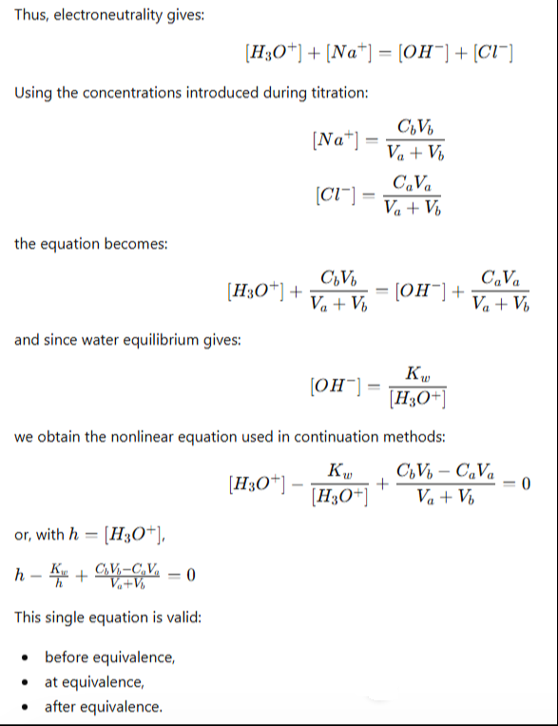
(*ElectroneutralityEquation:Unknowns:y=pHVb=addedbasevolumeHydroniumconcentration:h=10^-yStrongacid/basebalance:h-Kw/h+(CbVb-CaVa)/(Va+Vb)=0Thissingleequationremainsvalidbefore,at,andafterequivalence.*)system[{y_,Vb_},Ca_]:=Module[{h},h=10^-y;Cb=Ca;{h-Kw/h+(Cb*Vb-Ca*Va)/(Va+Vb)}];(*equivalencetakesplaceatVb=10mlsinceVa*Ca=Vb*Cb,Va=10mlandCb=Ca*)
In[]:=
(*Arc-lengthcontinuation*)arcLengthBranch[Ca_,ds_:0.15,nSteps_:250]:=Module[{curve={},sol,y0,Vb0,vars,J,tangent,predictor,corrector,yPred,VbPred,yNew,VbNew,eqs,i},(*initialpoint*)Vb0=0.;y0=-Log10[Ca];AppendTo[curve,{Vb0,y0}];(*Continuationloop*)Do[vars={y,Vb};(*Jacobianrowvector*)J=D[system[{y,Vb},Ca][[1]],{vars}]/.{y->y0,Vb->Vb0};(*tangentvectororthogonaltoJacobian*)tangent={-J[[2]],J[[1]]};tangent=Abs@tangent/Norm[tangent];(*enforcepositivedirectioninVb*)(*predictorstep*)predictor={y0,Vb0}+ds*tangent;yPred=predictor[[1]];VbPred=predictor[[2]];(*correctorstep*)eqs={system[{y,Vb},Ca][[1]]==0,tangent[[1]](y-yPred)+tangent[[2]](Vb-VbPred)==0(*arc-lengthhyperplaneconstraint*)};sol=Quiet@FindRoot[eqs,{{y,yPred},{Vb,VbPred}},MaxIterations->100];yNew=y/.sol;VbNew=Vb/.sol;If[NumericQ[yNew]&&NumericQ[VbNew]&&0<=VbNew<=Vbmax,AppendTo[curve,{VbNew,yNew}];y0=yNew;Vb0=VbNew];,{i,nSteps}];curve];
(*Computeallfourcurves*)branches=Table[arcLengthBranch[Ca],{Ca,CaList}];
In[]:=
(*plot*)plots=Table[ListLinePlot[branches[[i]],PlotRange->{{0,20},{0,14}},PlotStyle->{colors[[i]],Thick,Dashed},InterpolationOrder->2],{i,Length[branches]}];finalPlot=Show[plots,Frame->True,Axes->False,AspectRatio->1,FrameLabel->{Style["Vb (mL)",14],Style["pH",14]},PlotRange->{{0,20},{0,14}},GridLines->Automatic,ImageSize->400{1,1},PlotLabel->Style["Strong Acid / Strong Base Titration\n Ca=Cb and Va=10 ml",12,Darker@Red]](*TheaccuracyofthetitrationincreasesasthesolutionsbecomemoreconcentratedbecausethepHjumpattheequivalencepointbecomeslarger(seebluecurveforCa=0.1).*)