Perimeter of an Ellipse by Two Computational Methods
Authors: Housam Binous and Ahmed Bellagi
Perimeter of an Ellipse by Two Computational Methods
Authors: Housam Binous and Ahmed Bellagi
Authors: Housam Binous and Ahmed Bellagi
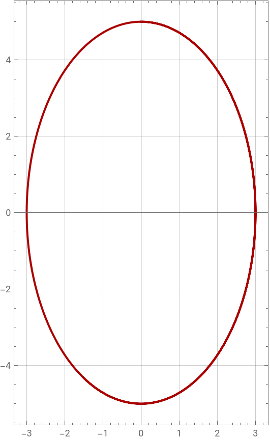
We compute the perimeter of an ellipse using two different approaches: (1) Elliptic integral formulation and (2) Arc-length continuation (numerical differential approach).The ellipse is defined by: +=1Method 1: Based on Elliptic IntegralThe exact perimeter of an ellipse is given by: where: E(m) is the complete elliptic integral of the second kind and e is the eccentricity defined as: .Method 2: Arc-Length Continuation MethodThe second approach is based on the definition of arc length, where the perimeter is computed as the total length of a parametric curve.For , both calculations yield
2
x
2
a
2
y
2
b
P=4bE()
2
e
e=
1-
2
a
2
b
a=3andb=5
P=25.527
Method based on elliptic integral
(*Semi-axes*)a=3;b=5;
(*Eccentricity*)e=Sqrt[1-(a^2/b^2)];
(*Exactperimeterusingellipticintegral*)Pexact=4.bEllipticE[e^2]
Out[]=
25.527
Method based on arc - length continuation
eq1=x[s]^2/a^2+y[s]^2/b^2==1(*equationofanellipse*)
Out[]=
2
x[s]
9
2
y[s]
25
eq2=x'[s]^2+y'[s]^2==1(*auxiliaryequation*)
Out[]=
2
′
x
2
′
y
In[]:=
SOL=Quiet@First@NDSolve[{eq1,eq2,x[0]==0,y[0]==b,x'[0]==0.01,y'[0]==0},{x,y},{s,0,40},AccuracyGoal->20]
Out[]=
xInterpolatingFunction,yInterpolatingFunction


In[]:=
ParametricPlot[{x[s],y[s]}/.SOL,{s,0,40},Frame->True,GridLines->Automatic,PlotStyle->Darker@Red,ImageSize->Medium]
Out[]=
In[]:=
P=s/.FindRoot[(x[s]/.SOL)==0,{s,25}]
Out[]=
25.527