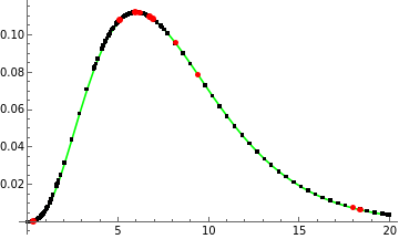
We could sample a function for "interesting" points (in red) by randomly sampling from the points (in black) that are chosen while plotting the PDF curve (in green).
In[]:=
func@x_=PDF[GammaDistribution[4,2],x]gr1=Plot[func@x,{x,0,20},PlotStyleGreen];pts=First@Cases[gr1,Line@pts_pts,Infinity];gr2=ListPlot[pts,PlotStyleRed];exactSample={#,func@#}&/@(Rationalize[#,10^-24]&@@@Sort@RandomSample[pts,10]);Show[gr1,ListPlot[pts,PlotStyleBlack],ListPlot[exactSample,PlotStyleRed]]
Out[]=
|
Out[]=
Here were the values of the interesting points that were chosen:
In[]:=
N@exactSample
Out[]=
{{0.331234,0.000320779},{5.09377,0.107832},{5.94439,0.112006},{6.18938,0.111857},{6.74895,0.109628},{6.93294,0.108396},{8.16628,0.0956128},{9.40392,0.0786358},{17.9601,0.00759735},{18.3567,0.00665289}}
For example, if we took the first red point, which is a pair of exact numbers,
In[]:=
N[example=First@exactSample,24]exactInputVal=First@example
Out[]=
{0.331233721551335657173351,0.000320778986235508122688611}
Out[]=
50872393
153584583
and expressed the x ordinate machine precision representation as an Interval
In[]:=
InputForm[inputInt=Interval@N@exactInputVal]
Out[]//InputForm=
Interval[{0.3312337215513356, 0.33123372155133574}]
We can see how that interval is transformed by the PDF function, func.
In[]:=
InputForm[outputInt=func@inputInt]
Out[]//InputForm=
Interval[{0.0003207789862355078, 0.00032077898623550843}]
We could also compare the output interval to the exact output via subtraction.
In[]:=
exactOutputVal=Last@exampleoutputInt-exactOutputVal
Out[]=
131657771883712185282457
347787606482698721153595552
50872393/307169166
Out[]=
Interval[{-2.71051×,3.79471×}]
-19
10
-19
10