What is the simplest universal non-deterministic Turing Machine? While proving universality is incredibly difficult, it is interesting to explore simple NDTMs to explore what kind of complex behaviour these exhibit. It has been proven that Wolfram’s 2-state 3-colour Turing Machine is universal, so perhaps a non-deterministic 2-state 2-colour machine with 5 rules is universal? In this project, I have developed various tools to visualise and analyse non-deterministic Turing Machines, so that we get a better understanding of their capabilities.
Overview
Overview
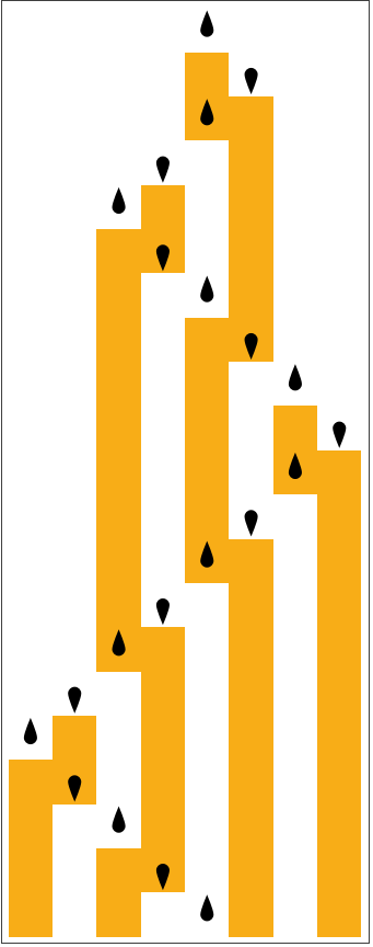
Turing Machines are the quintessential models of computation and have been studied extensively. In A New Kind of Science, Stephen Wolfram visualises and explores some of the simpler such machines. From a given set of rules, for instance:
In[]:=
RulePlot[TuringMachine[2506]]
Out[]=
we can easily trace the evolution of the machine:
In[]:=
RulePlot[TuringMachine[2506],{1,{{},0}},20]
Out[]=
However, it gets more challenging to effectively visualise this evolution with non-deterministic Turing Machines. If there is, for instance, two possible rules corresponding to the same case, we get a multiway system:
In[]:=
With[{t=3},Show[ResourceFunction["MultiwayTuringMachine"][{524,652},{{1,t+1,0},Table[0,2t+1]},t,"StatesGraph","IncludeEventInstances"->True,VertexSize->1.1{1,1/(2t+1)}]]/.Arrowheads[Medium]->Arrowheads[0.025]]
Out[]=
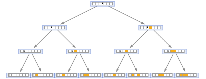
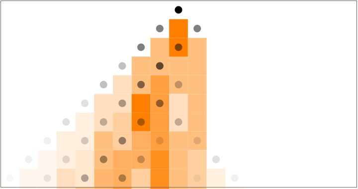
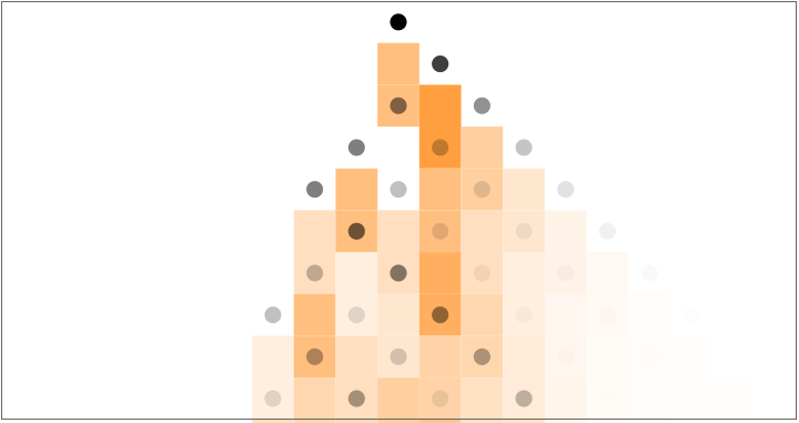
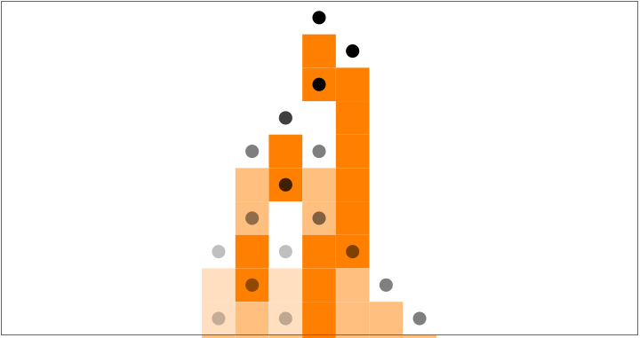
From such a graph, it is difficult to get an intuitive and holistic understanding of how the machine operates. We must, therefore, conceive of alternative ways of visualising NDTMs. One way is simply to average both the tape and the head positions. The different paths are weighted by the inverse of the number of times the path has bifurcated in branchial space. We can therefore interpret the resulting averaged tape and distribution of head positions as the probability when doing a random walk in branchial space of getting a configuration where the tape is coloured and the head is in that position. Below is the evolution of NDTM 39 189. As you can see, it has 5 rules. This means that it has a duplicate rule only for one case, while the remaining three cases are deterministic.
From such a graph, it is difficult to get an intuitive and holistic understanding of how the machine operates. We must, therefore, conceive of alternative ways of visualising NDTMs. One way is simply to average both the tape and the head positions. The different paths are weighted by the inverse of the number of times the path has bifurcated in branchial space. We can therefore interpret the resulting averaged tape and distribution of head positions as the probability when doing a random walk in branchial space of getting a configuration where the tape is coloured and the head is in that position. Below is the evolution of NDTM 39 189. As you can see, it has 5 rules. This means that it has a duplicate rule only for one case, while the remaining three cases are deterministic.
In[]:=
ndRulePlot[$allNTDMs[[39189]]]
Out[]=
In[]:=
plotHistory[limitedNdtmEvolution[$allNTDMs[[39189]],{{1,10,0},ConstantArray[0,20]},30,5]]
Out[]=
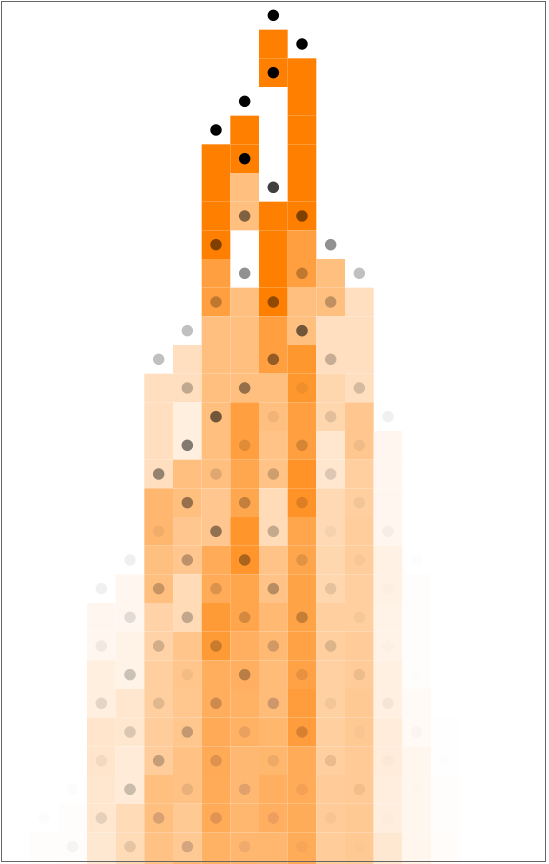
I have been working with the simplest NDTMs, namely those that have 2 states, 2 symbols, and 5 rules (such that there is only non-determinism in one of the four cases). There are in total 57 344 such machines. For each of the 4096 2-state 3-symbol TMs, there are 28 unused rules. However, simply multiplying these numbers will double count every machine, so we get =57344 distinct machines. If we take into account the symmetries from states, symbols, and the head movement, we are left with 7 168 machines.Naturally, not all of these exhibit as interesting behaviour, particularly when plotted on a blank tape. Here, for instance, is the “family” of TM 0:
4096×28
2
In[]:=
Multicolumn[plotFamilyOfTM[0,10]]
Out[]=
| |||||
|
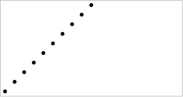
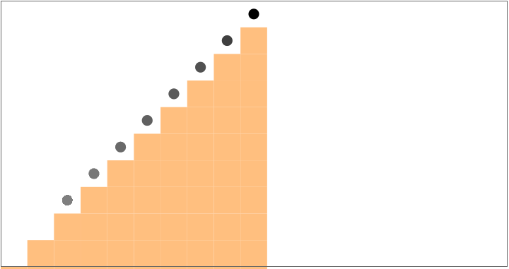
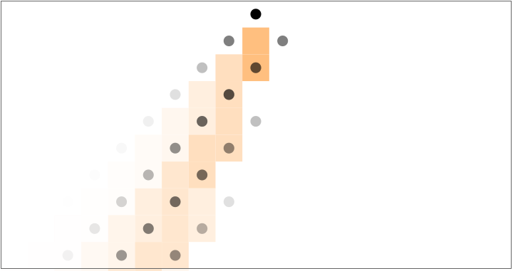
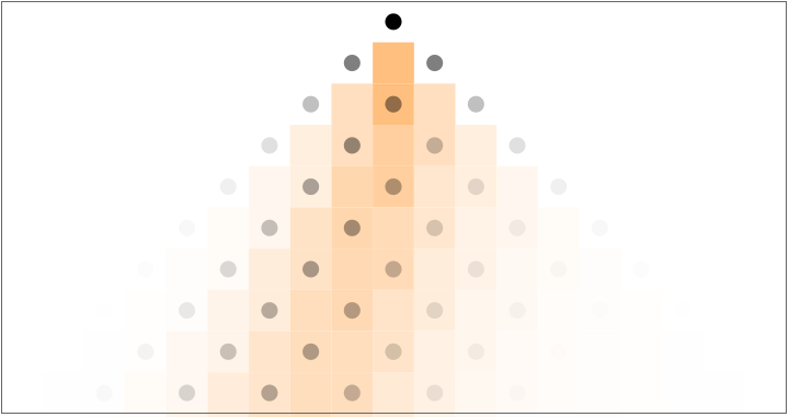
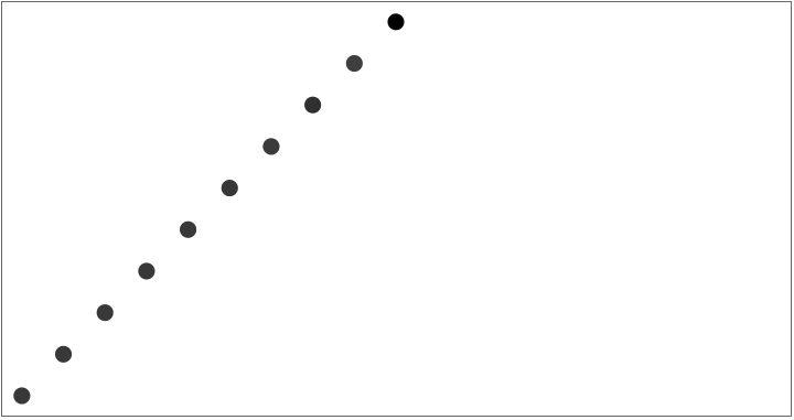
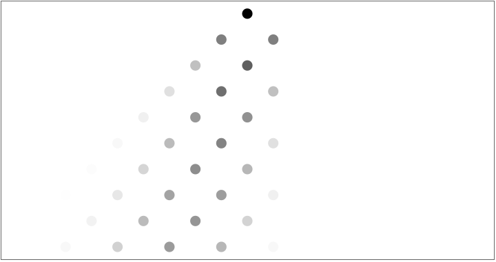
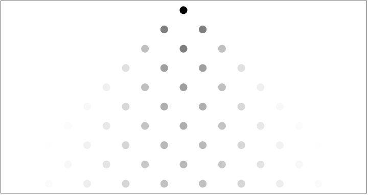
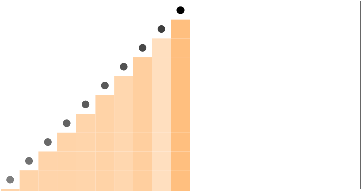
On the other hand, the family of TM 2506 has much more interesting behaviour:
In[]:=
Multicolumn[plotFamilyOfTM[2506,10]]
Out[]=
| |||||
|
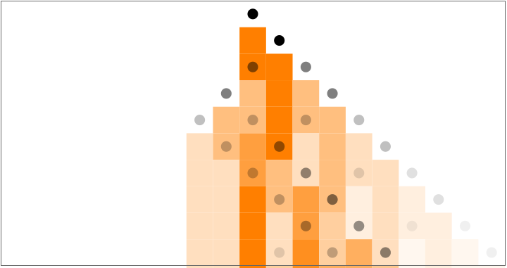
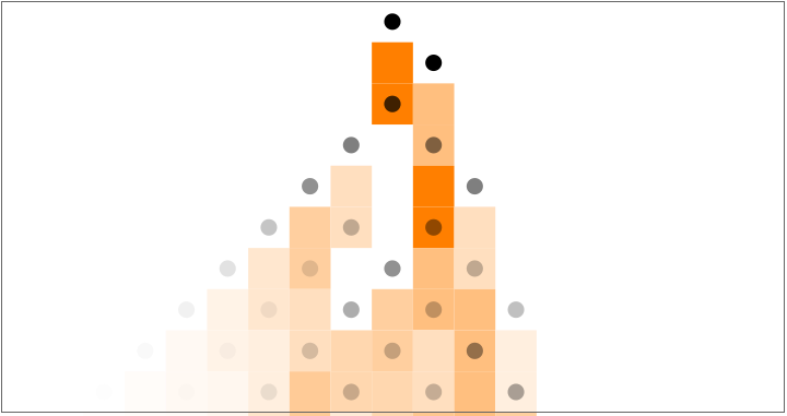
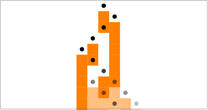
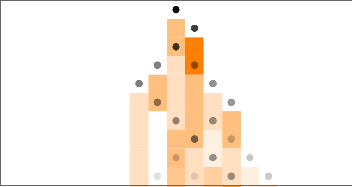
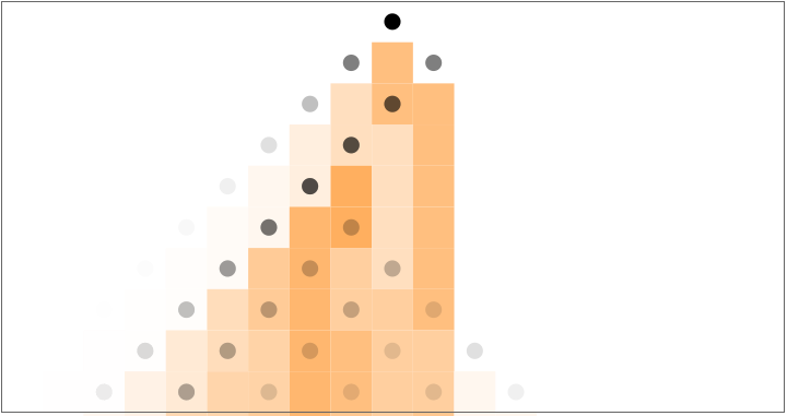
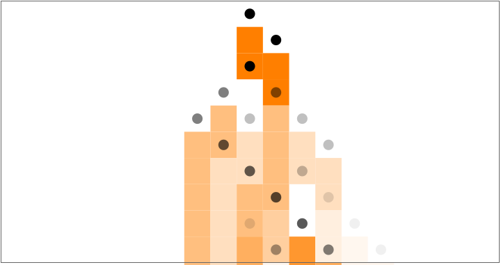
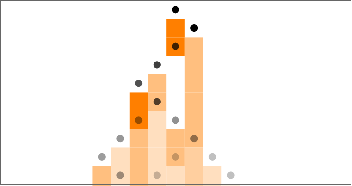
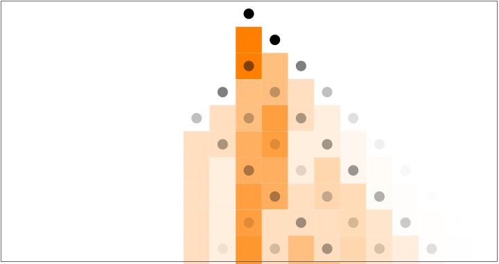
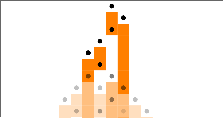
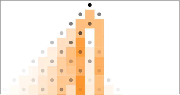
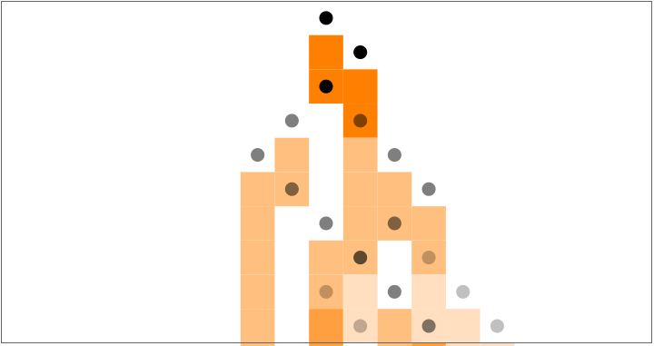
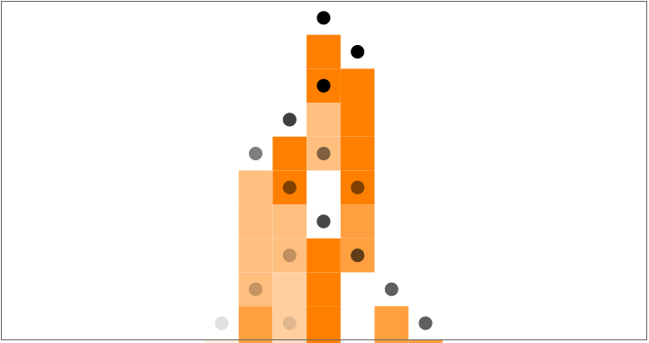
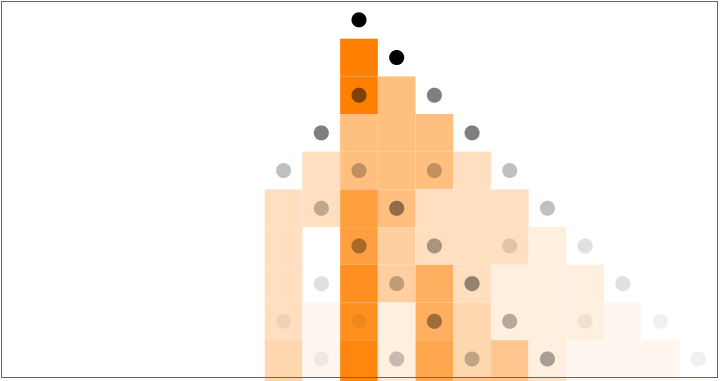
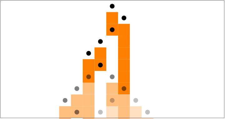
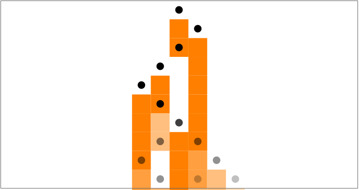
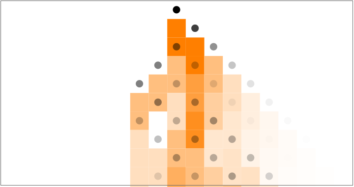
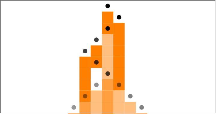
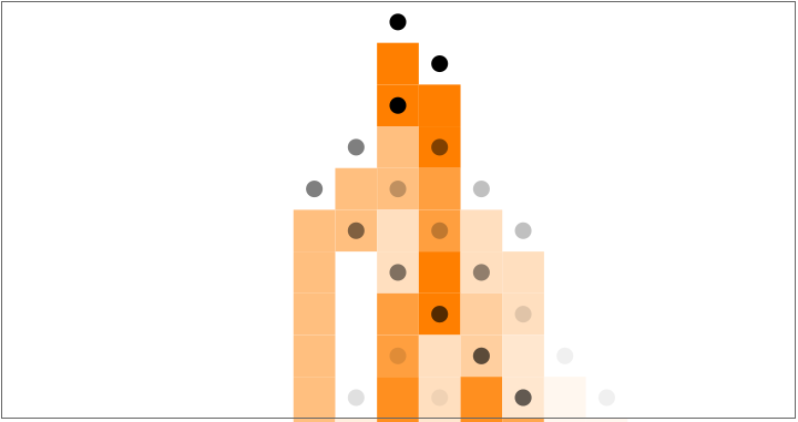
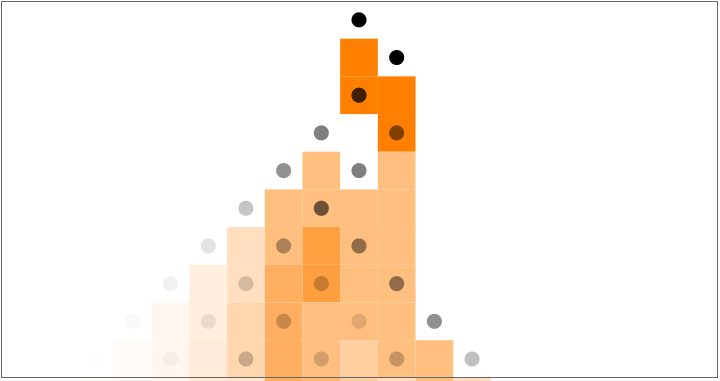
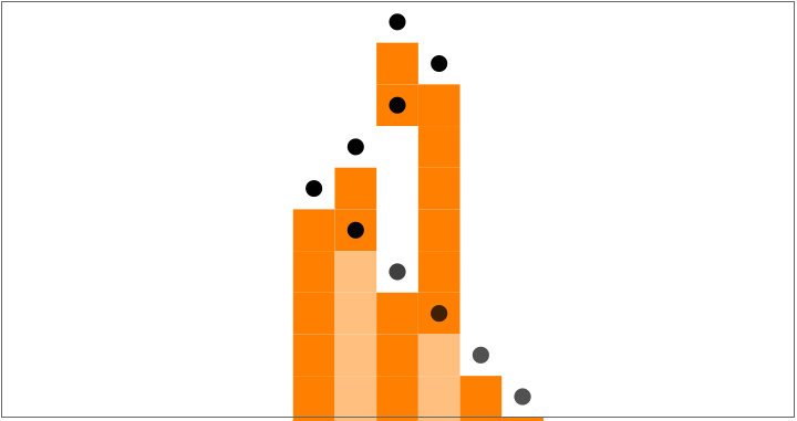
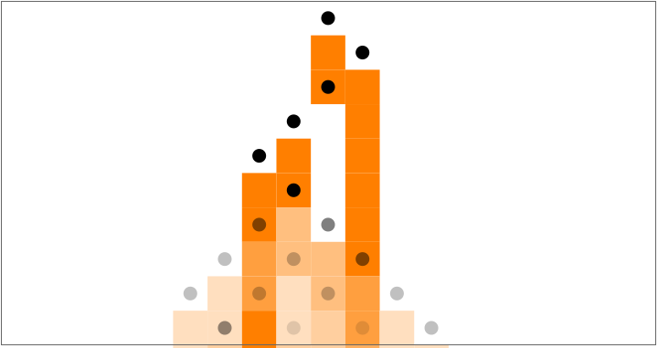
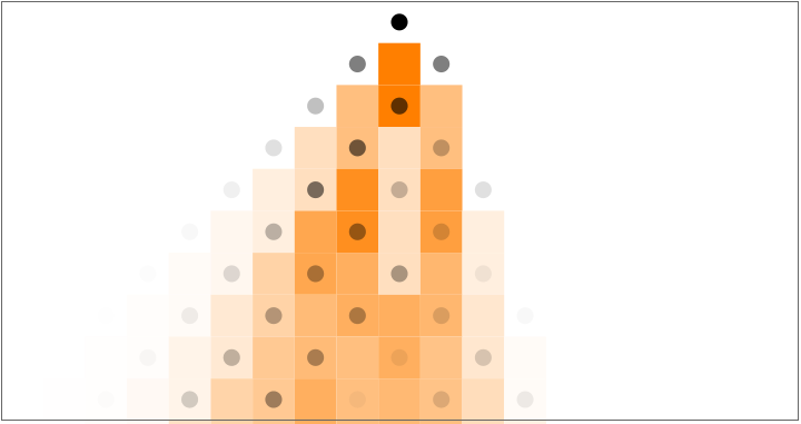
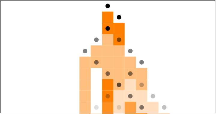
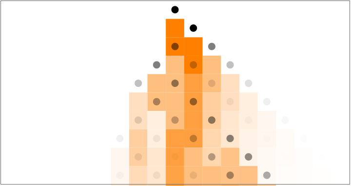
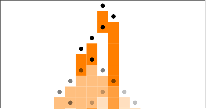
We can analyse the distribution of both tape configurations and head positions for all of the different NDTMs.
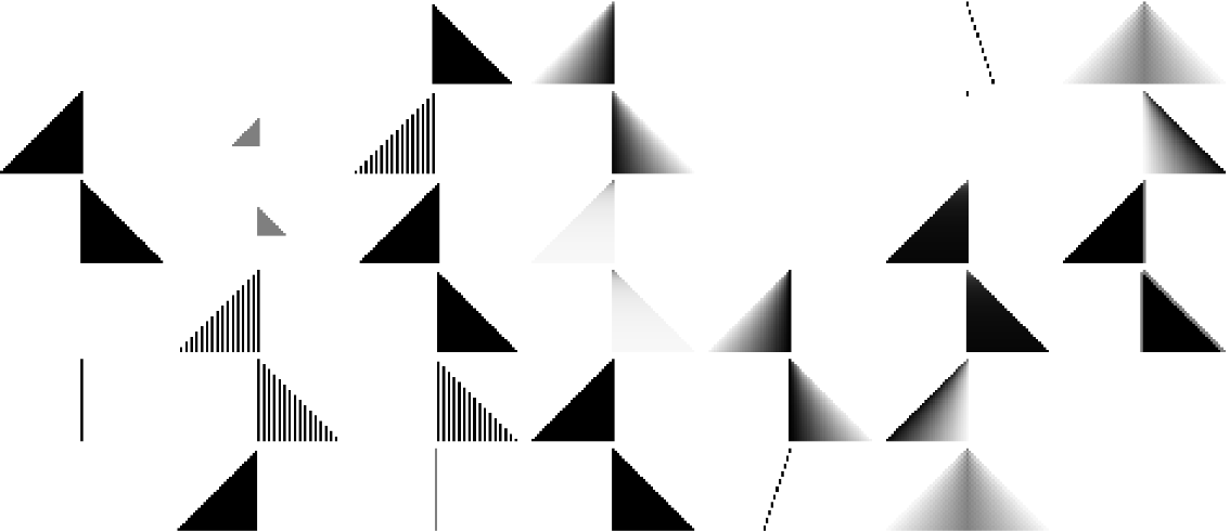
Here are the 40 most common (sorted by column) tape configurations after running the machine for 32 steps.
We can analyse the distribution of both tape configurations and head positions for all of the different NDTMs.
Here are the 40 most common (sorted by column) tape configurations after running the machine for 32 steps.
In[]:=
Multicolumn[Table[plotMeanTape[$tapeArrays[[$tapeGroups[[i,1]]]]],{i,1,40}]]
Out[]=
And some of the less common ones:
And some of the less common ones:
Branching
Branching
To more quantitatively analyse branching, we can plot the number of different head positions at the end of the simulation, or the distribution of head positions at every step. While this isn’t a perfect metric for branching (because there might be merges or paths with the same head position but different states/tapes), it is a good proxy for determining how much an NDTM branches.
As we see in the histogram and matrix plots, it is most commonly no branching at all, while there are small peaks at various powers of 2 (due to the exponential nature of the machines) as well as at n (the number of steps in the simulation, as many machines branch linearly). However, the most interesting machines are likely those who do not conform to any of these patterns, but have their own idiosyncratic evolution.
As we see in the histogram and matrix plots, it is most commonly no branching at all, while there are small peaks at various powers of 2 (due to the exponential nature of the machines) as well as at n (the number of steps in the simulation, as many machines branch linearly). However, the most interesting machines are likely those who do not conform to any of these patterns, but have their own idiosyncratic evolution.
Enumeration
Enumeration
Conclusion
Conclusion
From this preliminary analysis, I’m unfortunately unable to have any good intuition about whether some of these machines might be universal, and proving this is naturally even more difficult. But it remains clear that despite having such simple rules, these machines are able to exhibit a plethora of different complex behaviour, which warrants both appreciation as well as further investigation.
Further Research
Further Research
There is still need for further research in this field. Some possible directions to explore:
◼
Explore deeper the machines presented here to see whether any of them exhibit particularly interesting or complex behaviour and whether any of the machines are potential candidates for the simplest universal NDMT
◼
Develop alternative ways of visualising non-determinism, such as stacking different paths in three dimensions
◼
Performing similar analyses on more advanced Turing Machines. For instance exploring the behaviour of 3-state non-deterministic Turing Machines
◼
Examining how to intuitively average three symbols with a three-colour palette when analysing 3-symbol machines
◼
Performing similar analyses on more interesting initial configurations, such as non-blank (random) initial tape, or perhaps circular tapes
Code
Code
Keywords
Keywords
◼
Turing Machines
◼
Non-determinism
◼
Random Walks
◼
Branchial Space
Acknowledgments
Acknowledgments
Mentor: Taliesin Beynon
Thank you to Tali for his guidance to all aspects of this project as well as his massive help with implementing my ideas in the Wolfram language.
Thank you to Kiel Howe for his crash course in modern physics and hypergraphs that prepared me well for this summer school.
Thank you also to Stephen Wolfram for offering valuable feedback and an interesting project prompt, and to WSS 2020 for the opportunity to explore these interesting phenomena.
Thank you to Kiel Howe for his crash course in modern physics and hypergraphs that prepared me well for this summer school.
Thank you also to Stephen Wolfram for offering valuable feedback and an interesting project prompt, and to WSS 2020 for the opportunity to explore these interesting phenomena.