Preprint/Working Draft
This document is a preprint and working draft intended for community feedback.
It has not been peer-reviewed and has not been formally published.
© 2026 - Donald Airey. All rights reserved.
This work is intended for submission to a peer-reviewed journal.
Public posting of this draft does not constitute prior publication and does not waive the author’s right to publish a revised version.
Gravity and Action from the Evolution of a Complex Manifold
Gravity and Action from the Evolution of a Complex Manifold
A Kinematic Origin for Gravity, Action, and Cosmic Evolution
Abstract
Abstract
We present a bilocal geometric framework in which separations are defined between ordered pairs of events rather than by a local infinitesimal metric. This construction is motivated by the need to represent global evolution in a manner that remains well-defined over finite separations while admitting a smooth local limit. The resulting geometry is formulated on a complex manifold with an imaginary temporal coordinate and a real spatial coordinate. A constant manifold acceleration sets the global spatial scale and produces a parabolic cycle of expansion and contraction. In the local reduction, the same acceleration scale yields a circular-orbit envelope consistent with the baryonic Tully-Fisher relation. At cosmological scales, the resulting analytic distance--redshift relation predicts the Pantheon+ Type~Ia supernova luminosity distances on the SH0ES-calibrated absolute scale and yields a lower covariance-weighted than Planck-calibrated FLRW, without invoking dark matter or dark energy. The parabolic metric evolution, when combined with standard recombination microphysics, yields an acoustic angular scale consistent with Planck measurements.
2
χ
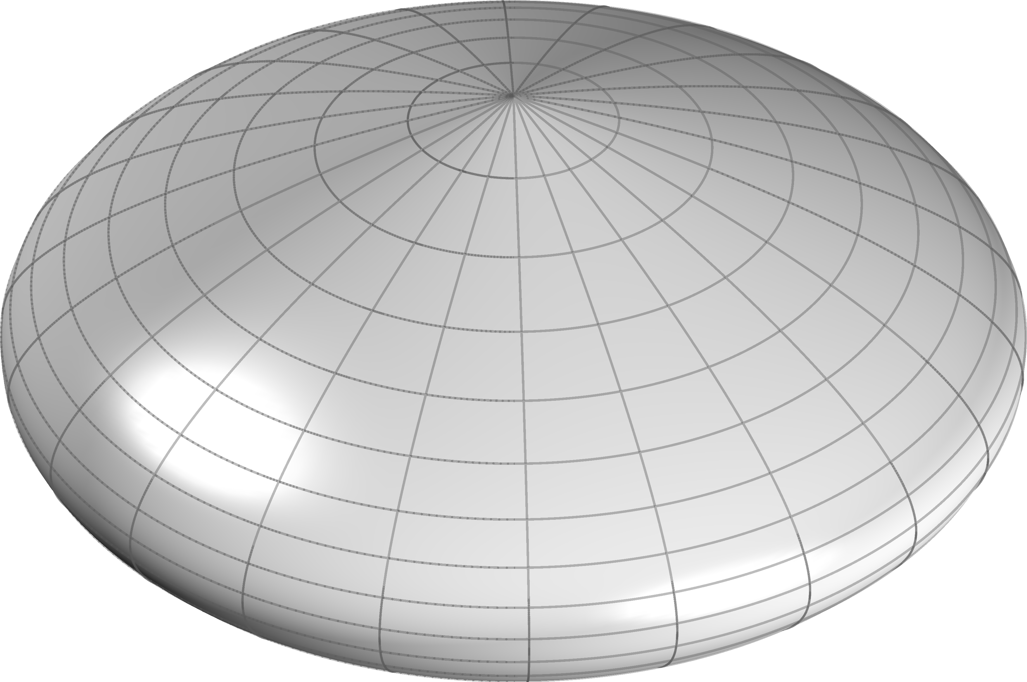
Figure 1. Schematic representation of the complex parabolic metric manifold. Latitude lines correspond to spatial slices at fixed epoch, while longitude lines trace the temporal evolution of the manifold.
Setup and Definitions
Setup and Definitions
Environment Cleanup
Environment Cleanup
Typesetting Rules
Typesetting Rules
Introduction
Introduction
Cosmological observations tightly constrain theoretical descriptions of the universe. Measurements of the cosmic microwave background (CMB) fix early-universe conditions and global geometry with high precision [1], while Type Ia supernovae (SNe Ia) probe the late-time expansion history through the luminosity distance-redshift relation [2]. Although each dataset is internally consistent, discrepancies arise when parameters inferred from early- and late-time observations are compared. In particular, the tension in the Hubble constant [1, 3] indicates that the standard cosmological model may be incomplete.
Historically, such discrepancies have been addressed by extending the model. The cosmological constant was introduced to permit a static universe [4] and abandoned following the discovery of expansion [5]. Galaxy rotation curves motivated the introduction of non-baryonic dark matter [6], and supernova evidence for accelerated expansion led to the reintroduction of the cosmological constant as dark energy [7, 8]. While these additions yield a phenomenologically successful framework, the dominant components of the cosmic energy budget remain physically unexplained [1]. More recent approaches introduce additional degrees of freedom, including time-varying dark energy [9], further increasing the parametric structure of the model.
We develop a kinematic framework in which large-scale evolution and local gravitational phenomena arise from a common geometric structure, termed the Parabolic Metric Evolution (PME). Local metric descriptions specify infinitesimal separations, so finite separations between distant events must be constructed by integrating along a chosen connection; in a globally evolving system, this construction can depend on both the path and the evolution of the geometry. The PME framework replaces this path-dependent procedure with a bilocal definition that assigns separations directly to ordered event pairs while admitting a consistent local limit. Motion on the manifold is governed by a single intrinsic kinematic scale, eliminating the need for multiple independent cosmological parameters and linking global expansion and local dynamics to a common geometric origin. The geometric structure of the manifold is illustrated in Fig. 1.
This approach differs from relativistic metric gravity in its bilocal definition of separation and from modified-gravity models [10, 11] in that the characteristic acceleration scale is not introduced phenomenologically but inherited from the global manifold kinematics by the local-reduction regime. Cosmological evolution, gravity, and the laws governing motion are thereby unified through a single acceleration scale determined by the manifold kinematics.
The resulting construction defines a minimal kinematic closure: the lowest-order geometric structure that consistently relates finite separations, global evolution, and local dynamics within a single framework, without introducing independent dynamical components. The bilocal definition of separation provides a representation of finite intervals compatible with global evolution, and the restriction to a single intrinsic acceleration scale selects the simplest nontrivial homogeneous dynamics beyond uniform motion, yielding a closed and self-consistent description across cosmological and local regimes.
Bilocal Geometry
Bilocal Geometry
Foundational Structure
Foundational Structure
The framework is defined by the following postulates:
1
.Physical separations are defined bilocally between ordered pairs of events.
2
.The manifold evolution is governed by a constant acceleration scale .
A
3
.The manifold is parameterized by an intrinsic evolution coordinate .
χ
4
.Observable time is defined operationally through null exchange, providing an invariant ordering of events. The intrinsic evolution parameter is related to this observable time by the projection , which fixes the real-imaginary decomposition of temporal and spatial functionals and serves as a defining structural postulate of the framework.
χit
All subsequent results follow from this structure.
Bilocal Spatial Separation
Bilocal Spatial Separation
Let , denote an emission event and , an observation event, with the bilocal interval constructed from a temporal functional obtained from accumulated evolution between slices and a spatial functional defined from separations on the emission and observation slices.
p
e
0
x
e
1
x
e
p
o
0
x
o
1
x
o
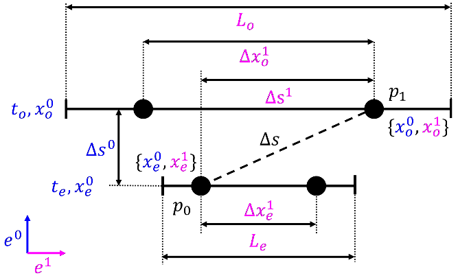
Figure 2. Geometric construction of the bilocal interval between emission event and observation event , showing the accumulated temporal evolution and the symmetric midpoint spatial separation between scaled slices.
p
e
p
o
The bilocal construction is illustrated in Figure 2. The spatial slices scale with a global manifold extent , so the separations at emission and observation satisfy
L(t)
1
Δx
e
L[]
t
e
1
Δx
o
L[]
t
o
(
1
)In[]:=
comovingRelation=;
1
Δx
e
L[]
t
e
1
Δx
o
L[]
t
o
Imposing symmetry under interchange of emission and observation together with a smooth coincidence limit motivates adopting the midpoint average as the minimal symmetric choice,
ΔΔ-Δ-Δ
1
s
1
x
o
1
2
1
x
o
1
x
e
(
2
)ΔΔ+Δ
1
s
1
2
1
x
o
1
x
e
(
3
)In[]:=
1
Δs
1
Δx
o
1
2
1
Δx
o
1
Δx
e
Out[]=
1
2
1
Δx
e
1
Δx
o
Invariance of the Bilocal Interval
Invariance of the Bilocal Interval
Consider a bilocal scalar constructed from the temporal and spatial endpoint functionals . We adopt a quadratic form as the lowest-order scalar consistent with finite separations, ensuring that the local reduction yields a well-defined null condition while avoiding higher-order dependence on endpoint structure,
(Δ,Δ)
0
s
1
s
Δa+b+2cΔΔ
2
s
2
(Δ)
0
s
2
(Δ)
1
s
0
s
1
s
(
4
)Under interchange of the ordered endpoints , the temporal functional changes sign while the symmetric spatial functional does not, so the mixed term changes sign. Invariance therefore requires .
(,)
p
e
p
o
c0
In the local reduction, sufficiently small endpoint separations render the temporal and spatial functionals linear in the coordinate increments. The null condition must define a finite null ratio, which requires both temporal and spatial contributions to enter non-degenerately so that the null condition defines a finite null ratio. The interval therefore reduces to
Δa+b
2
s
2
(Δ)
0
s
2
(Δ)
1
s
The remaining quadratic form is therefore constrained up to a positive overall factor and a relative scaling between the temporal and spatial functionals. These functionals are not arbitrary coordinates but are identified with the canonical imaginary and real components of the complex manifold, with this identification fixing their relative normalization. The bilocal interval is therefore
Δ+
2
s
2
(Δ)
0
s
2
(Δ)
1
s
(
5
)In[]:=
2
Δs
2
()
0
Δs
2
()
1
Δs
with purely imaginary and real.
Δ
0
s
Δ
1
s
Imaginary Velocity
Imaginary Velocity
The intrinsic evolution of the manifold is parameterized by a coordinate . Observable time is introduced by the projection , so that , fixing the real-imaginary decomposition used in the bilocal construction.
χ
χit
dχit
In[]:=
χ[t_]=t;
Withconstantintrinsicacceleration,thevelocityscalealongthemanifoldhistoryfollowsfromintegrationwithrespectto,
A
χ
v(t)∫Aχ
Substituting gives , which evaluates to
dχit
v(t)i∫At
v(t)i(At-)
V
0
(
6
)In[]:=
v[t_]=Simplify∫Aχ[t]t-
∂
t
V
0
Out[]=
(-+At)
V
0
where is an integration constant representing the initial expansion rate of the manifold.
V
0
Induced Spatial Evolution
Induced Spatial Evolution
The observable spatial extent arises from integrating the imaginary velocity along the imaginary temporal direction. The global spatial scale of the manifold is therefore . Substituting the expression for and using gives . Evaluating the integral yields
L(t)≡∫v(t)χ
v(t)
dχit
L(t)∫i(At-)it
V
0
L(t)t-A
V
0
1
2
2
t
(
7
)In[]:=
L[t_]=∫v[t]χ[t]t
∂
t
Out[]=
V
0
A
2
t
2
Manifold Deceleration
Manifold Deceleration
The intrinsic evolution is defined along , while observable dynamics are expressed in the projected time coordinate with . Rewriting the manifold extent in terms of yields its observable form. Differentiating twice with respect to gives
χ
t
dχit
t
t
Cosmological Distance
Cosmological Distance
Observable cosmological distances follow from the bilocal interval defined in equation (5).
Temporal Separation
Temporal Separation
Evaluating the integral yields
The temporal separation is purely imaginary and depends only on the endpoints.
Spatial Separation
Spatial Separation
Solving equation (1) for the emission separation gives
Bilocal Metric Formula
Bilocal Metric Formula
Substituting the temporal and spatial separations into equation (5) yields the interval relating the emission and observation events,
Redshift Relation
Redshift Relation
Redshift is defined observationally by the ratio of observed to emitted wavelength,
Causal Structure
Causal Structure
Differentiating the causal horizon gives the expansion rate of the causal boundary,
This quantity defines the rate at which the accessible causal domain can be extended under the operational clock, and therefore characterizes the growth of the causally orderable region.
The causal horizon is therefore twice the manifold extent at all epochs, placing the entire last-scattering surface within a single causal region. Because the homogeneous manifold acceleration introduces no preferred direction, the large-scale isotropy of the cosmic microwave background follows directly from the geometry.
Gravity
Gravity
Coincidence Limit
Coincidence Limit
Using the local expansion of the manifold extent,
the slice-separation relation gives
Hence
so the bilocal spatial component becomes
Substituting these leading terms into equation~(\ref{eq:bilocal_interval}) yields
Acceleration Field
Acceleration Field
The effective inward acceleration in a bound system decomposes into a homogeneous background and a sourced concentration,
Minimal Local Closure
Minimal Local Closure
For a spherically symmetric configuration the sourced acceleration is radial,
Imposing flux conservation together with linearity in the enclosed inertial content gives
and Gauss’s theorem gives
Circular Orbits
Circular Orbits
Equating this with the inward acceleration from equation (27) gives
Then, solving for the enclosed baryonic mass gives
Circular-Orbit Solutions
Circular-Orbit Solutions
The mass therefore reaches a maximum at
Baryonic Tully-Fisher Relation
Baryonic Tully-Fisher Relation
A characteristic acceleration scale in galaxy dynamics has previously been emphasized in frameworks such as MOND [10], in which the force law is modified to reproduce Tully-Fisher-type scaling.
The best-fit manifold acceleration is
Global Acceleration Budget
Global Acceleration Budget
Using the global relation between baryonic mass and the background acceleration scale,
yields
Regularity of the Manifold
Regularity of the Manifold
Because the manifold acceleration scale is finite, collapse approaches saturated configurations of finite density and radius rather than singular limits. The manifold accordingly remains smooth under the evolution defined by the geometry and does not admit singular collapse.
Causal ordering is fixed by the intrinsic geometry of allowable separations, not by any imposed signal speed. Only trajectories consistent with this ordering admit an operational time parameter, excluding closed timelike curves and the associated causal paradoxes.
The causal structure and finite acceleration budget thereby avoid singularities and causal paradoxes.
Newton’s Bucket
Newton’s Bucket
Newton’s rotating-bucket argument establishes that the concavity of the water surface cannot be attributed to rotation relative to the bucket, and therefore requires a standard of rotation not reducible to the relative configuration of nearby bodies. Mach proposed that this standard is supplied by the aggregate distribution of distant matter, so that rotation would lose physical meaning in an otherwise empty universe. General relativity does not adjudicate between these positions: the field equations admit solutions in which local inertial frames align with the mean matter distribution, and solutions such as the Gödel universe in which the matter congruence rotates relative to the local inertial structure. In the latter case a bucket at rest with respect to the cosmic matter exhibits a concave surface, while a suitably rotating bucket exhibits a flat one. The outcome of the experiment is therefore a property of the choice of solution, not a prediction of the theory.
Local Dynamics
Local Dynamics
Having established the gravitational and causal structure, we now define the operational dynamics governing motion within the manifold.
Operational Time
Operational Time
so that
The null relation therefore fixes the local causal structure and operational ordering of events. Observable motion and the invariant timelike interval both arise from this same local geometry, so causality, motion, and measurable duration are unified through the null structure of the manifold.
Proper Time
Proper Time
Using the local interval defined in equation (25),
giving
Local Momentum
Local Momentum
Momentum is defined from the observable velocity,
Local Action
Local Action
defines the invariant geometric action increment,
with quadratic form
Using the local invariant
the action-space interval becomes
The temporal component defines the geometric energy scale associated with tangent evolution,
and therefore
so that the invariant geometric action accumulates along the manifold tangent,
Observable action is obtained by projection into the timelike sector,
which defines the canonical momentum and observable Hamiltonian. The observable action therefore plays the role of the Hamilton-Jacobi principal function, while the invariant geometric action remains well-defined across the full manifold.
Phase Evolution
Phase Evolution
The continued evolution of this invariant scalar is represented as phase,
where ℏ sets the scale relating geometric action to phase. Because action has units of length within the present framework, ℏ acquires the interpretation of a minimum indivisible bilocal separation, a necessary structural feature of a geometry that does not admit infinitesimal separations.
Phase evolution therefore represents the continuation of invariant geometric evolution beyond the proper-time-parametrized sector, while the underlying manifold evolution remains continuous across the null boundary.
Late-Time Evolution
Late-Time Evolution
The distance-redshift relation derived from the bilocal interval predicts the late-time expansion history.
Type Ia Supernova Sample
Type Ia Supernova Sample
Luminosity Distance
Luminosity Distance
Distance Modulus
Distance Modulus
Type Ia supernova observations are reported in terms of the distance modulus, which relates the observed luminosity distance to the measured brightness of each supernova,
Manifold Kinematic Parameters
Manifold Kinematic Parameters
The local null scale at the observation epoch is
The best-fit observation epoch is obtained by minimizing the covariance-weighted chi-square statistic
Table 1 - PME kinematic parameters determined from BTFR and Cepheid-calibrated Pantheon+ subset.
Comparison with Observations
Comparison with Observations
Figure 5 shows the PME prediction and the Planck 2018 FLRW model compared with the Pantheon+SH0ES data.
The resulting covariance-weighted chi-square values are
Figure 5. Pantheon+SH0ES distance moduli with PME (red) and spatially flat FLRW (blue) predictions evaluated on the same absolute calibration. Lower panel shows residuals relative to each model.
Hubble Function
Hubble Function
The Hubble constant therefore emerges as a prediction rather than a fitted parameter.
Cosmic Time
Cosmic Time
The redshift–time relation differs from standard cosmological evolution due to the underlying parabolic evolution. Table II compares the resulting cosmic times with those from FLRW algorithms.
The parabolic expansion yields uniformly larger cosmic ages than FLRW, significantly extending the available time for early structure formation.
Table II - Cosmic time as a function of redshift. PME predictions are compared with FLRW values computed using Planck 2018 parameters.
Early-Time Evolution
Early-Time Evolution
Independent constraints arise from the cosmic microwave background (CMB), whose acoustic scale probes the distance to last scattering relative to the sound horizon.
The expansion history is determined by the PME kinematics derived above, while recombination microphysics is evaluated using standard rate equations. Thermodynamic quantities are mapped using the scale factor
Baryon and Photon Densities
Baryon and Photon Densities
The recombination history and pre-decoupling sound speed require the baryon and photon densities. The baryon density is fixed by the manifold acceleration scale rather than introduced as an independent cosmological parameter. This follows from the local divergence law (equation (33)), which relates the sourced acceleration field to the baryonic density.
hence
Using the kinematic parameters determined in the previous sections yields
This value is consistent with independent observational estimates of the present-day baryon density from primordial light-element abundances [13].
and, following the geometric sign convention of Eq. (58), the mean photon energy is
The corresponding photon energy density is
so the mass-equivalent photon density becomes
These densities determine the baryon-photon momentum ratio and the free-electron density entering the visibility function.
Recombination Epoch
Recombination Epoch
The recombination epoch is the time of maximum photon visibility, i.e. the most probable last-scattering time in the baryon-photon plasma.
The Thomson scattering rate is expressed in terms of the local particle density, cross section, and local geometric scale,
The corresponding visibility function is
Sound Horizon
Sound Horizon
The baryon–photon momentum ratio is defined as
giving the sound speed
Acoustic Angular Scale
Acoustic Angular Scale
Using the redshift relation from equation (15), this becomes
The corresponding effective transverse radius is
The acoustic angular scale is then
Evaluating this expression with the manifold parameters gives
Expressed in the conventional CMB notation,
This result follows from the PME expansion geometry combined with standard recombination microphysics.
Conclusion
Conclusion
A constrained bilocal construction on a complex manifold yields a quadratic interval whose local reduction yields a homogeneous acceleration scale. This single geometric scale governs both the parabolic evolution of the manifold and the redistribution of acceleration flux in gravitationally bound systems. The bilocal geometry produces an emergent local null constraint, defines an invariant action geometry, and admits a canonical decomposition into temporal and spatial contributions. From this structure, a Hamiltonian system and associated Hamilton--Jacobi equation arise as the projection of the inertia-weighted invariant geometric action into the timelike sector, so that particle motion follows geodesics of action space without introducing independent dynamical postulates, while phase evolution provides its continuation beyond the observable domain. Gravity and inertia therefore emerge as complementary manifestations of a conserved acceleration field inherited from the manifold kinematics.
The evolution implied by this construction yields a closed analytic distance-redshift relation, from which the Pantheon+ Type Ia supernova luminosity distances follow directly on an absolute scale. The same parameter set predicts the present-day Hubble constant and produces uniformly extended cosmic ages. In the local-reduction regime, redistribution of the homogeneous acceleration field generates an inverse-square sourced component and a circular-orbit envelope consistent with the observed baryonic Tully-Fisher relation. The acceleration scale inferred from galaxy dynamics then fixes the baryonic density of the homogeneous universe, linking galactic and cosmological observables without introducing non-baryonic dark matter or dark energy components.
The bilocal construction also determines the causal horizon and implies a constant ratio between the causal domain and manifold extent, placing the last-scattering surface within a single causal region and accounting for large-scale isotropy. The geometry yields a transverse scale for recombination that reproduces the observed acoustic angular scale. Because the available acceleration flux is finite, gravitational collapse approaches saturated configurations, eliminating curvature singularities and enforcing a globally ordered causal structure. Rotational inertia emerges from redistribution of the same finite acceleration budget, providing a Machian interpretation in which local inertial behavior depends on the global distribution of inertial content.
Evolution, causal structure, action, gravity, inertia, and dynamical law therefore arise from a common bilocal origin, with all dynamics derived from the momentum weighted invariant separation, providing a unified explanation of isotropy, galaxy rotation, Type~Ia supernova magnitudes, the acoustic scale, nonsingular gravitational collapse, the baryonic density, and the Hubble constant.
References
References
[1] Planck Collaboration, N . Aghanim, et al. Planck 2018 results. vi. cosmological parameters. Astronomy & Astrophysics, 641: A6, 2020.
[2] Dillon Brout, Dan Scolnic, Boian Popovic, Adam G . Riess, et al. The Pantheon + analysis: Cosmological constraints from 1701 Type Ia supernovae. Astrophysical Journal, 938(2):110, 2022.
[3] Adam G.Riess, Wenlong Yuan, Lucas M.Macri, et al. A comprehensive measurement of the local value of the Hubble constant. Astrophysical Journal Letters, 934: L7, 2022.
[4] A.Einstein. Kosmologische betrachtungen zur allgemeinen relativit¨atstheorie. Sitzungsberichte der Koniglich Preußischen Akademie der Wissenschaften, pages 142–152, 1917.
[5] Edwin Hubble. A relation between distance and radial velocity among extra-galactic nebulae. Proceedings of the National Academy of Sciences,15(3):168–173,1929.
[6] Vera C.Rubin, W.Kent Ford, and Norbert Thonnard. Rotational properties of 21 SC galaxies with a large range of luminosities and radii. Astrophysical Journal,238:471–487,1980.
[7] Adam G . Riess, Alexei V . Filippenko, Peter Challis, et al. Observational evidence from supernovae for an accelerating universe and a cosmological constant. Astronomical Journal, 116 : 1009–1038, 1998.
[8] Saul Perlmutter, Greg Aldering, Gerson Goldhaber, et al. Measurements of Omega and Lambda from 42 high-redshift supernovae. Astrophysical Journal, 517 : 565–586, 1999.
[9] Eleonora Di Valentino, Alessandro Melchiorri, Joseph Silk, et al. In the realm of the Hubble tension—a review of solutions. Classical and Quantum Gravity, 38 (15) : 153001, 2021.
[10] Mordehai Milgrom. A modification of the Newtonian Dynamics as a possible alternative to the hidden mass hypothesis. Astrophysical Journal, 270 : 365–370, 1983.
[11] Stacy S . McGaugh, Federico Lelli, and James M . Schombert. Radial acceleration relation in rotationally supported galaxies. Physical Review Letters, 117 : 201101, 2016.
[12] Stacy S . McGaugh, James M . Schombert, Gregory D . Bothun, and W . J . G . de Blok . The baryonic tully–fisher relation . Astrophysical Journal Letters, 533 : L99–L102, 2000.
[13] R . J . Cooke, M . Pettini, K . M . Nollett, and R . Jorgenson . The primordial deuterium abun - dance of the most metal - poor damped lyman - α system . Astrophysical Journal, 830 : 148, 2016.