In this notebook, we present a “Manipulate” demonstration of orbits around a Schwarzschild black hole. The demonstration lets us explore the parameter space of a test “star” orbiting a black hole, at-will constructing stable orbits with relativistic precession or crashing the star into the event horizon, never to return.
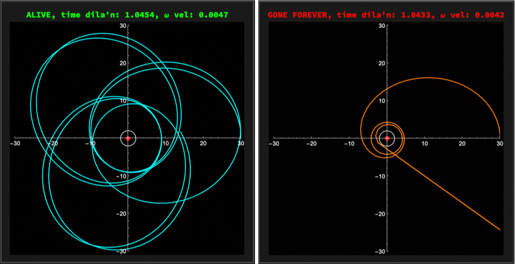
A good way to read this notebook is to page to the end, play with the demonstration, then read the leading prose explaining the physics.
The solutions are built on the compiler proof-of-concept presented in earlier notebooks. We take advantage of the Schwarzschild metric from the Wolfram Function Repository, but compute the Christoffel symbols (force-producers), ab-initio, in . From the Christoffel symbols, we posit the standard equations of motion for coordinates of the star in terms of proper time τ:
2
d
μ
x
d
2
τ
μ
Γ
νλ
d
ν
x
dτ
d
λ
x
dτ
In a future notebook, we’ll compute the Schwarzschild metric ab-initio, also. For now, it’s more interesting to show the visualizations.
Initialize Toolkit and Compiler
Initialize Toolkit and Compiler
Optional: Quit for a Fresh Kernel
Optional: Quit for a Fresh Kernel
◼
Note, if you call Quit in a notebook, evaluation may hang. If you want to “Evaluate Notebook,” mark the following cell “Evaluatable” in the CellProperty menu, call Quit once, then comment out the Quit cell, or mark it unevaluatable again. Alternatively, you can quit the kernel via the Evaluation menu (last item). At that point, you can “Evaluate Notebook” in a clean environment. Otherwise, you can evaluate cells in this notebook individually.
->
(*CellisnotEvaluatablebydefault*)Quit[];
In[]:=
RTbranch="main";RTbase="https://raw.githubusercontent.com/rebcabin/RelativityToolkit/"<>RTbranch<>"/";RTbust="?t="<>ToString[Round[AbsoluteTime[]]];(*Forcefreshdownload*)RTrules=RTbase<>"RelativityToolkit.wl"<>RTbust;RTSchwarzschildCompilerPoc=RTbase<>"APPLICATION_SCRIPTS/schwarzschild_compiler_poc.wl"<>RTbust;Get[RTrules];Get[RTSchwarzschildCompilerPoc];
»
Relativity Toolkit version :1.9.0
»
Relativity Connection Symbol :Γ
Orbits
Orbits
Imagine a spherical coordinate system measuring time and spatial locations, , θ, ϕ, stretching out from the center of a supermassive black hole to a safe distance, where spacetime is almost flat. Launch a star, as a test particle of negligible mass, to orbit the black hole. Spacetime is highly curved close to the black hole, but relativity gives us the way to figure out what our “flat” coordinates will read as we measure time and locations from our safe distance.
t
r
Integrate the equations of motion of the star as a function of its proper time. The star follows geodesics around the black hole. If the star gets too close to the event horizon at (in natural units, ), the star will disappear from the Universe forever, suffering an unknowable fate, perhaps at the singularity in the center of the black hole.
r=2
M
blackhole
G=c=1
Define Unknown Functions of τ
Define Unknown Functions of τ
In[]:=
coords={t,r,θ,ϕ};funcs={t[τ],r[τ],θ[τ],ϕ[τ]};velocities=D[funcs,τ];
Build ODEs from the Compiled Γ Array
Build ODEs from the Compiled Γ Array
The following is a straight transcription of the standard equations of motion:
2
d
μ
x
d
2
τ
μ
Γ
νλ
d
ν
x
dτ
d
λ
x
dτ
(
1
)via myGammaArray from the compiler script.
◼
Note the resemblance to Newton’s , if we interpret the term with the connection Γ as producing forces. This idea is so pervasive in all of physics that it deserves a slogan: Forces Come from Connections. We’ll see it again in gauge theory in future notebooks, where the connections, instead of describing curvature of spacetime, describe curvatures in symmetry groups of gauge fields.
F=ma
◼
TODO: Derive these equations as describing geodesics, ab-initio, from a variational principle.
In[]:=
(odes=Table[(D[funcs[[μ]],{τ,2}]+Sum[myGammaArray[[μ,ν,λ]]*velocities[[ν]]*velocities[[λ]],(*myGammaArrayindicesare1-based*){ν,1,4},{λ,1,4}]==0)//FullSimplify,{μ,1,4}])//TableForm
Out[]//TableForm=
2M. ′ r ′ t 2 r. ′′ t |
(r.-2M.)M. 2 ′ t 3 r. ′′ r M. 2 ′ r 2 r. 2 ′ θ 2 Sinθ. 2 ′ ϕ |
Cosθ.Sinθ. 2 ′ ϕ 2 ′ r ′ θ r. ′′ θ |
2 ′ r ′ θ ′ ϕ r. ′′ ϕ |
Substitute Unknown Functions for Formals in Γ
Substitute Unknown Functions for Formals in Γ
The proof-of-concept compiler uses formal symbols as variables. This artifact is inherited from the Wolfram Function Repository, the target “virtual machine” of the compiler, and propagates the formal symbols back up.
Map the formal symbols to our unknown functions for NDSolve’s sake. Set the black hole’s mass, , to 1, arbitrarily (the mass will have the same units as , the radial distance, so about solar masses if length is measured in light-seconds). Solve the equations algebraically into state-space form for inspection, with accelerations all to the left of equals signs.
M
r
2×
5
10
In[]:=
odes=odes/.r.->r[τ],θ.->θ[τ],ϕ.->ϕ[τ],t.->t[τ]//TableForm;nums=M.->1;(odes=Solve[odes,D[funcs,{τ,2}]][[1]]/.{Rule->Equal}/.nums)//Column
Out[]=
′′ t 2 ′ r ′ t (2-r[τ])r[τ] |
′′ r 2 ′ r -2r[τ]+ 2 r[τ] (-2+r[τ]) 2 ′ t 3 r[τ] 2 ′ θ 2 Sin[θ[τ]] 2 ′ ϕ |
′′ θ -2 ′ r ′ θ 2 ′ ϕ r[τ] |
′′ ϕ 2( ′ r ′ θ ′ ϕ r[τ] |
Smoke Test
Smoke Test
The following parameters are known empirically to produce a stable-ish orbit.
In[]:=
Mval=1;rStart=14;ecc=0.98;(*slightellipse*)
Initial Angular Velocity ϕ
Initial Angular Velocity
ϕ
From balancing Newtonian gravitational force against centripetal force
GMm
2
r
m
2
v
r
M
r
(
2
)in natural units, .
G=c=1
◼
This condition is usually good enough for a stable Newtonian orbit, but not good enough for Einstein; you can still crash a star into a black hole with this initial condition, as we see later.
Multiply it by the eccentricity and divide again by to get initial angular velocity of our elliptical orbit:
r
(ϕ')
0
In[]:=
phiVel=
ecc
rStart
Mval
rStart
Out[]=
0.0187083
Initial Coordinate Time
Initial Coordinate Time
There is heavy time dilation near the black hole. That means that coordinate time will be highly non-linear w.r.t. τ and is subject to numerical integration. A good initial value for , given the initial angular velocity phiVel above, comes from the requirement that the proper velocity, υ, always have negative unit norm:
dt/dτ
u.υ=-1=+
g
tt
2
(t')
0
g
ϕϕ
2
(ϕ')
0
(
3
)There are no and terms because we always start with pure planar motion =0 and no radial speed =0.
g
θθ
g
rr
(θ')
0
(r')
0
◼
TODO experiment with non-zero initial radial speed in a new Manipulate.
In the Schwarzschild metric, becomes
υ.υ
-1-+(ϕ')=-1
2M
r
0
2
t'
0
2
2
r
0
0
(
4
)producing
t'
0
1+(ϕ')
2
2
r
0
0
1-
2M
r
0
(
5
)In[]:=
tVel=
1+
2
rStart
2
phiVel
1-2Mval/rStart
Out[]=
1.11656
Final System to Solve
Final System to Solve
In[]:=
inits={t[0]==0,t'[0]==Echo[tVel,"initial time vel"],r[0]==Echo[rStart,"initial (apo/peri)apsis"],r'[0]==0,θ[0]==π/2,θ'[0]==0,(*STRICTLYPLANAR*)ϕ[0]==0,ϕ'[0]==Echo[phiVel,"initial ang vel"]};finalSystem=Join[odes,inits];
Run Simulation
Run Simulation
Extreme effects of relativity are on display as precession.
◼
The 2020 Nobel Prize in Physics was awarded for measuring the mass of the supermassive black hole at the center of our Milky Way galaxy by tracking the highly elliptical orbit of the star S2. Later, measuring the orbit’s precession further verified general relativity.
Visualize Simulation Bookends
Visualize Simulation Bookends
Interactive Black-Hole Lab
Interactive Black-Hole Lab
Interesting Things to Try
Interesting Things to Try
Interactive Reparameterization
Interactive Reparameterization
Precession Scrub
Precession Scrub
With the default parameters (press the RESET button), scrub the duration forward and backward slowly to watch the precession. Try the animation tools in the duration control at various speeds. The animation may be blocky at times, but if you pause the animation, the orbit eventually (and quickly) smooths out. This is a design feature of the animator: it prioritizes latency over fidelity just the same way your browser will sometimes give you a blocky image at first and then refine it progressively over time.
Delicate Escape
Delicate Escape
At duration 130, you can see the “star” spiraling into the black hole. It doesn’t have enough ω to escape. By duration 135, it’s gone forever.
Increase the duration to the maximum (5000) and see the orbit surviving, probably forever.
Nearly Periodic Trifoil Precession
Nearly Periodic Trifoil Precession
Conclusion
Conclusion
In previous posts on the calculus, we focused on building the machinery: defining tensors, algebraic structures, and prototyping a compiler. In this post, we step back from just building the tool and use it for astrophysical science.
The best part of this experiment is what we didn’t have to do. To simulate the extreme environment of a Schwarzschild black hole, where space-time curves, time slows, and orbits precess, we did not write new physics code. We simply fed the Schwarzschild metric into our existing compiler, cranked out the Christoffel symbols, and let the standard geodesic equation do the rest.
In the Smoke Test, we metaphorically reproduce the famous Precession of the Perihelion of Mercury around the Sun, just with a much heavier orbit-producing black hole. In the Manipulate demonstration, we can push parameters to probe the Innermost Stable Circular Orbit (ISCO) and visually confirm our test star vanishes from the Universe at the event horizon.
This exercise confirms that is solid, so far. It can serve as a foundation for exploring more complex geometries such as the Kerr metric, and ventured in future posts into quantum gauge theories.
For now, please enjoy the Interactive Lab. Crash some stars, search for resonances in precession, and explore the fearsome math of general relativity.
References
References
1
.Beckman, Brian. From the steam age to quantum fields: a unified approach via UD tensorial calculus. Wolfram Community post.
2
.3
.4
.5
.6
.7
.[MTW] Misner, Charles W.; Thorne, Kip S.; Wheeler, John Archibald. Gravitation. Princeton University Press, 2017.
8
.Genzel, R., & Ghez, A., Mass Measurement via S2 Orbit. 2020 Nobel Prize in Physics.
9
.Detection of Precession: GRAVITY Collaboration. (2020). “Detection of the Schwarzschild precession in the orbit of the star S2 near the Galactic centre massive black hole.” Astronomy & Astrophysics.
10
.CITE THIS NOTEBOOK
CITE THIS NOTEBOOK
Interactive black hole dynamics in
by Brian Beckman
Wolfram Community, STAFF PICKS, February 2, 2026
https://community.wolfram.com/groups/-/m/t/3632176
by Brian Beckman
Wolfram Community, STAFF PICKS, February 2, 2026
https://community.wolfram.com/groups/-/m/t/3632176