
Calculate the transmitted & reflected energy balance through a single-layer etalon cavity.
Calculate the transmitted & reflected energy balance through a single-layer etalon cavity.
Model Assumptions:
Model Assumptions:
◼
The incident E field is an idealized monochromatic plane wave.
◼
The material stack consists of 3 layers, }, with layer forming the etalon cavity.
{,,
n
1
n
2
n
3
n
2
◼
The incident wave is assumed to enter from within layer .
n
1
◼
All media are characterized purely by their refractive indices, }, which may be either purely real or complex-valued.
{,,
n
1
n
2
n
3
◼
All dielectric materials are non-absorbing at the input λ.
◼
Hence, the range of permissible values for λ is may be implicitly restricted.
◼
All boundaries between adjacent media are plane-parallel surfaces.
◼
All media are isotropic & homogenous.
◼
The responses of all media to the incident field are assumed to be linear wrt the field intensity.
Unit conversion functions:
Unit conversion functions:
In[]:=
NDegtoRad[x_]:=QuantityMagnitude[x]*;NRadtoDeg[x_]:=x*;
π
180
180
π
AOI & Cavity Layer Definitions:
AOI & Cavity Layer Definitions:
In[]:=
n:={1.0,1.641,1.50+0I};λ:=633;numPts:=90;θ:=Range[0,numPts];d:=;
Range[0,numPts]
10
Intermediate Results:
Intermediate Results:
In[]:=
ν:=,;:=ArcSin[ν[[2]]];:=NRadtoDeg[ArcTan[ν[[1]]]];ϕ[x_]:=ArcSin,
n[[2]]
n[[1]]
n[[3]]
n[[2]]
θ
crit
θ
Brewster
NDegtoRad[x]
ν[[1]]
|
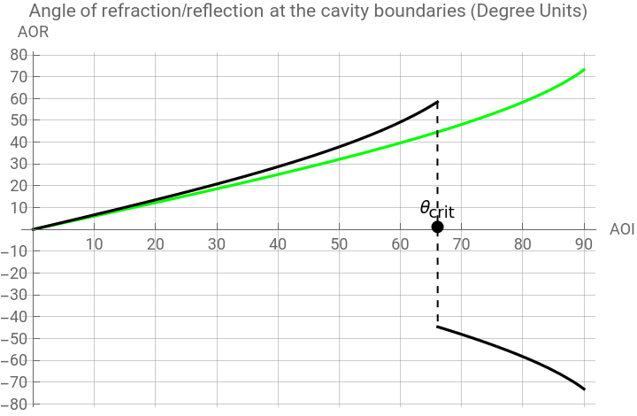
Calculate & Plot the Angle of Incidence (AOI) at The Cavity Boundary12&Boundary23.
Calculate & Plot the Angle of Incidence (AOI) at The Cavity &.
Boundary
12
Boundary
23
In[]:=
{ν,θ,NRadtoDeg[],,ϕ[θ]}
θ
crit
θ
Brewster
Out[]=
In[]:=
Plot{NRadtoDeg[ϕ[x][[1]]],NRadtoDeg[ϕ[x][[2]]]},{x,Min[θ],Max[θ]},PlotPoints->Automatic,PlotRange->Full,PlotStyle->{Green,Black},Exclusions->Automatic,ExclusionsStyle->{Dashed},PlotLegends->{"",""},PlotLabel->"Angle of refraction/reflection at the cavity boundaries (Degree Units)",AxesLabel->{"AOI","AOR"},AxesOrigin->{0,-Max[θ]},Ticks->{Range[QuantityMagnitude[-Max[θ]],QuantityMagnitude[Max[θ]],10]},GridLines->{Range[QuantityMagnitude[-Max[θ]],QuantityMagnitude[Max[θ]],10]},EpilogPointSize[Large],Point,[][[1]],Inset"",,Center
AOR
12
AOR
23
NRadtoDeg[]
θ
crit
r
tm
θ
crit
θ
crit
NRadtoDeg[]
θ
crit
Out[]=


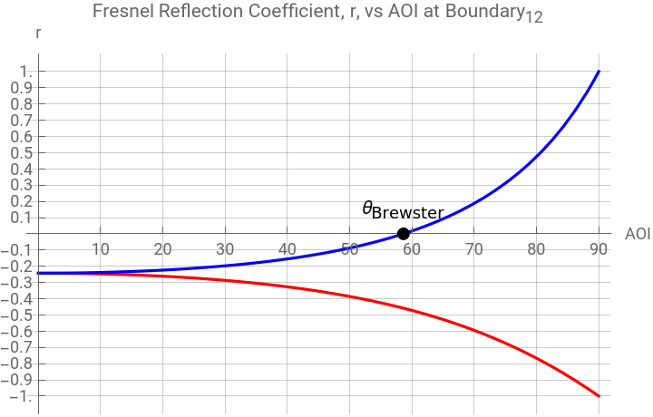
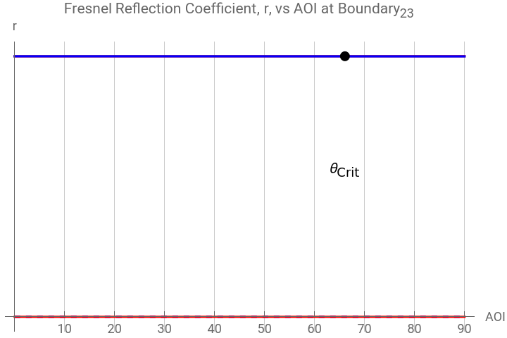
Calculate & Plot the Fresnel reflection coefficients at the cavity boundaries :
Calculate & Plot the Fresnel reflection coefficients at the cavity boundaries :
In[]:=
r
tm
-*Cos[x]+-
2
ν[[1]]
2
ν[[1]]
2
Sin[x]
2
ν[[1]]
2
ν[[1]]
2
Sin[x]
|
|
r
te
Cos[x]--
2
ν[[1]]
2
Sin[x]
Cos[x]+-
2
ν[[1]]
2
Sin[x]
|
|
In[]:=
Plot{[NDegtoRad[x]][[1]],[NDegtoRad[x]][[1]]},{x,Min[θ],Max[θ]},PlotPoints->Automatic,PlotRange->Full,PlotStyle->{Red,Blue},Exclusions->Automatic,ExclusionsStyle->{Dashed},PlotLegends->{"",""},PlotLabel->"Fresnel Reflection Coefficient, r, vs AOI at ",AxesLabel->{"AOI","r"},Ticks->{Range[QuantityMagnitude[Min[θ]],QuantityMagnitude[Max[θ]],10],Range[-1,1,0.1]},GridLines->{Range[QuantityMagnitude[Min[θ]],QuantityMagnitude[Max[θ]],10],Range[-1,1,0.1]},EpilogPointSize[Large],Point,[NDegtoRad[]][[1]],Inset"",,Center
r
te
r
tm
r
te12
r
tm12
Boundary
12
θ
Brewster
r
tm
θ
Brewster
θ
Brewster
θ
Brewster
Out[]=


In[]:=
Plot{[NDegtoRad[x]][[2]],[NDegtoRad[x]][[2]],[NDegtoRad[x]][[3]],[NDegtoRad[x]][[3]]},{x,Min[θ],Max[θ]},PlotPoints->Automatic,PlotRange->Full,PlotStyle->{Red,Blue,{Red,Dashed,Blue,Dashed}},Exclusions->Automatic,ExclusionsStyle->{Dashed},PlotLegends->{"Re[]","Re[]","Im[]","Im[]"},PlotLabel->"Fresnel Reflection Coefficient, r, vs AOI at ",AxesLabel->{"AOI","r"},Ticks->{Range[QuantityMagnitude[Min[θ]],QuantityMagnitude[Max[θ]],10],Range[-1.0,1.0,0.1]},GridLines->{Range[QuantityMagnitude[Min[θ]],QuantityMagnitude[Max[θ]],10],Range[-1.0,1.0,0.1]},AxesOrigin->{0,-Max[θ]},EpilogPointSize[Large],Point,[][[2]],Inset"",,Center
r
te
r
tm
r
te
r
tm
r
te23
r
tm23
r
te23
r
tm23
Boundary
23
NRadtoDeg[]
θ
crit
r
te
θ
crit
θ
Crit
NRadtoDeg[]
θ
crit
Out[]=


In[]:=
r
tm
Out[]=