
Modeling the aircraft longitudinal dynamics
Modeling the aircraft longitudinal dynamics
The dynamics are dictated by the equations describing the accelerations acting on the principal axes of the aircraft, since we are only taking into account the longitudinal dynamics for this example, we only need the equations for the horizontal and vertical accelerations in addition to the torque acting around the center of mass which changes the aircraft’s pitch angle.
◼
The horizontal acceleration is given by:
In[]:=
′
u
w
0
x
u
x
w
θ
0
x
δe
δ
e
◼
The vertical acceleration is given by:
In[]:=
′
w
u
0
z
u
z
w
θ
0
z
δe
δ
e
◼
The torque affecting the pitch angle:
{[t]q[t]+u[t]+w[t]+[t],[t]q[t]};
′
q
m
q
m
u
m
w
m
δe
δ
e
′
θ
Since the equations are non-linear, we can obtain a non-linear state space model of the aircraft:
aircraft=NonlinearStateSpaceModel,{u[t],w[t],q[t],θ[t]},[t],θ[t],t,SystemsModelLabels/.
δ
e
Out[]=

forward speed | u[t] | -0.00643u[t]+0.0263w[t]-32.2θ[t] |
vertical speed | w[t] | 0.+830q[t]-0.0941u[t]-0.624w[t]-32.7 δ e |
pitch rate | q[t] | -0.668q[t]-0.000222u[t]-0.00153w[t]-2.08 δ e |
pitch angle | θ[t] | q[t] |
pitch angle | θ[t] |
Controller Design
Controller Design
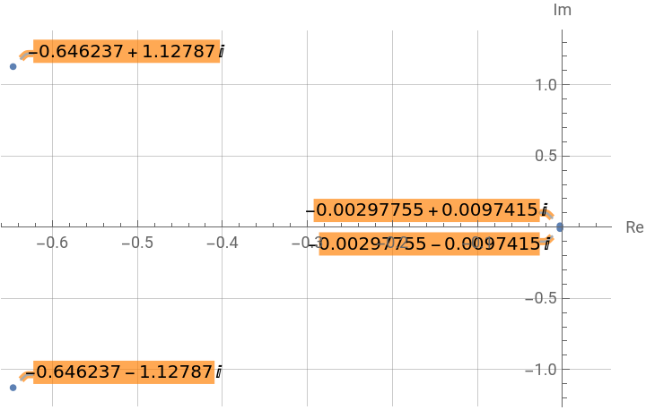
Before designing the controller, it is useful to gauge the stability of the uncompensated system. The pole-zero plot indicates that the system is marginally stable, meaning that this aircraft is unlikely to be flown safely without a stability augmentation system (SAS):
With[{p=TransferFunctionPoles[TransferFunctionModel[aircraft]][[1,1]]},ListPlot[Table[Callout[ReIm[p[[i]]],p[[i]],BackgroundOrange],{i,4}],PlotMarkers->{Automatic,5},GridLinesAutomatic,AxesLabel{Re,Im}]]
Out[]=
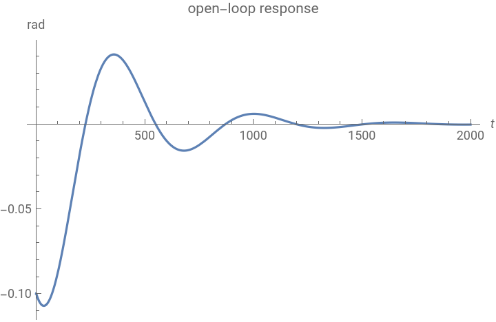
To assess the stability in terms of the dynamics, we can perturb the system away from it’s equilibrium state and simulate the response. Here the system is initialized with a disturbance in the pitch angle, and takes about seconds to stabilize which is very slow (and hence undesirable) for an aircraft:
1500
OutputResponse[{aircraft,{0,0,0,-0.1}},0,{t,0,2000}];Plot[%,{t,0,2000},PlotRangeAll,AxesLabel{t,rad},AxesLabel{t,rad},PlotLabel"open-loop response"]
Out[]=
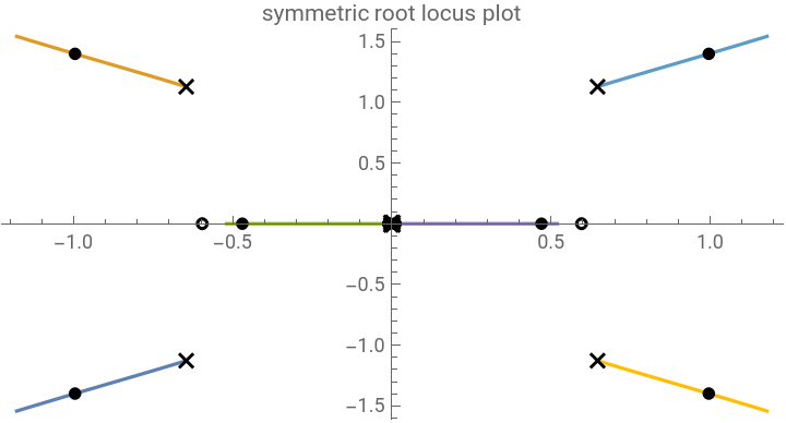
Designing an optimal controller requires the minimization of the integrand ρc.cx+ut, where ρ is the control weight and is the output matrix. We can use the symmetric root locus method to choose the optimal gains. The symmetric root locus is an efficient method to obtain the optimal gains as their effect on the poles can be visualized directly on a root locus plot:
∞
∫
0
2
(t)
2
(t)
symTFM=With[{tfm=TransferFunctionModel[aircraft,s]},tfm[s]tfm[-s]][[1,1]];symRLPlot=RootLocusPlot[ρsymTFM,{ρ,0,2.5},AspectRatio1/2,PlotLabel"symmetric root locus plot"]
Out[]=
The non linear state space model does not contain an output matrix. However, we can linearize the model to obtain a standard state space model and design the controller using the gains from the symmetric root locus plot, using StateSpaceModel:
aircraft=StateSpaceModel[aircraft]
Out[]=

| | elevator angle | |||
forward speed | -0.00643 | 0.0263 | 0 | -32.2 | 0 |
vertical speed | -0.0941 | -0.624 | 830 | 0 | -32.7 |
pitch rate | -0.000222 | -0.00153 | -0.668 | 0 | -2.08 |
pitch angle | 0 | 0 | 1 | 0 | 0 |
pitch angle | 0 | 0 | 0 | 1 | 0 |
The optimal controller data object can now be obtained using LQRegulatorGains:
c=Normal[aircraft][[3]];=With[{ρ=2.5},LQRegulatorGains[aircraft,{ρc.c,{{1}}},"Data"]]
Out[]=
SystemsModelControllerData


The closed-loop poles can be obtained as a property from the controller data object:
["ClosedLoopPoles"];%//MatrixForm
Out[]//MatrixForm=
-1.17886-1.54255 |
-1.17886+1.54255 |
-0.519898+0. |
-0.0104741+0. |
To increase the robustness of the controller, we can connect it to an estimator. The estimator gains can be obtained using EstimatorGains:
ℓ=EstimatorGains[aircraft,{-2+3,-2-3,-1,-0.05}];%//MatrixForm
Out[]//MatrixForm=
65793.9 |
-10028.7 |
10.6813 |
3.75157 |
Now that we have an optimal controller and estimator, we can assemble an estimator regulator controller for the aircraft:
E=EstimatorRegulator[aircraft,{ℓ,},"Data"]
Out[]=
SystemsModelControllerData

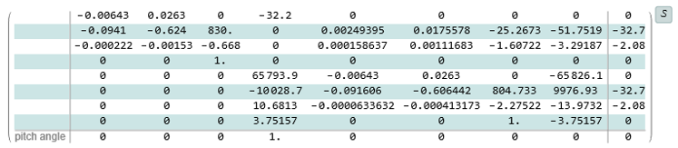
The closed-loop system for the aircraft with the estimator-regulator in the feedback path:
csys=E["ClosedLoopSystem"]//Chop
Closed-loop Performance and Results
Closed-loop Performance and Results
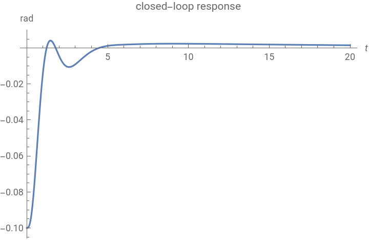
Let’s now assess the performance of the aircraft with the controller. We simulate the system with the same initial conditions as before and we notice there is a massive improvement in the performance:
or=OutputResponse[{csys,PadRight[{0,0,0,-0.1},8]},0,{t,0,20}];Plot[or,{t,0,20},PlotRangeAll,AxesLabel{t,rad},PlotLabel"closed-loop response"]
Out[]=
We can visualize how the system model poles have been displaced by placing the controller in the feedback path, which resulted in incrementing the system’s desirable performance characteristics:
Such performance gains could be too good to be feasible! It is indispensable to gauge the controller effort in order to be sure that it is reasonable: