Design of a two adiabatic packed bed system
Authors: Housam Binous and Ahmed Bellagi
Design of a two adiabatic packed bed system
Authors: Housam Binous and Ahmed Bellagi
Authors: Housam Binous and Ahmed Bellagi
Reference :
O. Levenspiel, Chemical Reaction Engineering, 3rd Edition, Wiley, 1999.
O. Levenspiel, Chemical Reaction Engineering, 3rd Edition, Wiley, 1999.
A system of two catalyst filled packed bed reactors is to be designed using the method of maximization of rectangles, the optimum conversion versus temperature data and the rate expression for exothermic reversible first order reactions.
This problem was solved graphically by O.Levenspiel in page 440 of Chemical Reaction Engineering, 3 rd Edition, Wiley, 1999.
We show how one can take advantage of the numerical and graphical features of Mathematica in order to rapidly solve this example.
Among the results obtained are catalyst weight in the two packed beds, heat duties of the three heat exchangers, temperature and conversions in all points of the system
Off[General::spell1]
Off[InterpolatingFunction::dmval]
R=8.314;
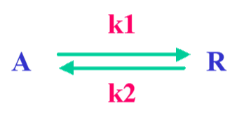
Exothermic Reversible first order reaction
Rate constants
k
1
k
2
Initial concentration of component A.
Pressure is 2.494 MPa.
Pressure is 2.494 MPa.
C
0
Heat of reaction
ΔH=-80000;
Rate of reaction
Rate=(1-X)-X;
k
1
C
0
k
2
C
0
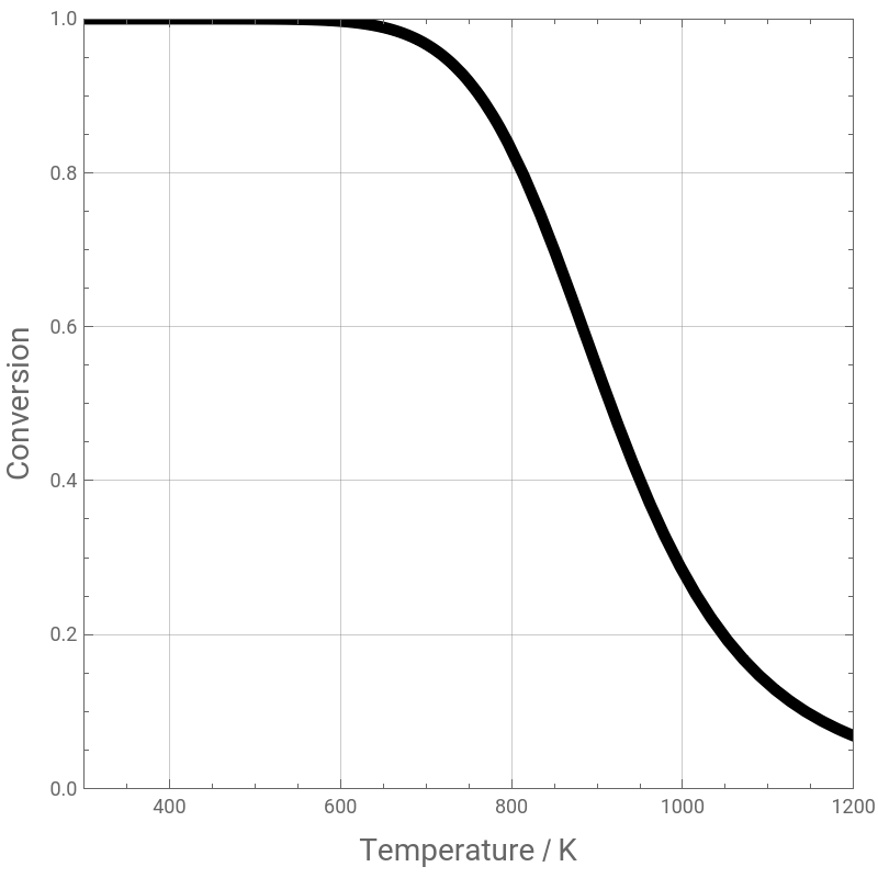
Equilibrium conversion versus temperature ( case when reaction rate equals zero ).
sol=Solve[Rate0,X];
plt=Plot[X/.sol,{T,300,1200},PlotStyle->{Thickness[0.015],RGBColor[0,0,0]},AspectRatio-> 1,FrameLabel->{Style["Temperature / K",14],Style["Conversion",14]},
ImageSize-> 400 {1,1},PlotRange->{{300,1200},{0,1}},Frame->True,GridLines->Automatic]
ImageSize-> 400 {1,1},PlotRange->{{300,1200},{0,1}},Frame->True,GridLines->Automatic]
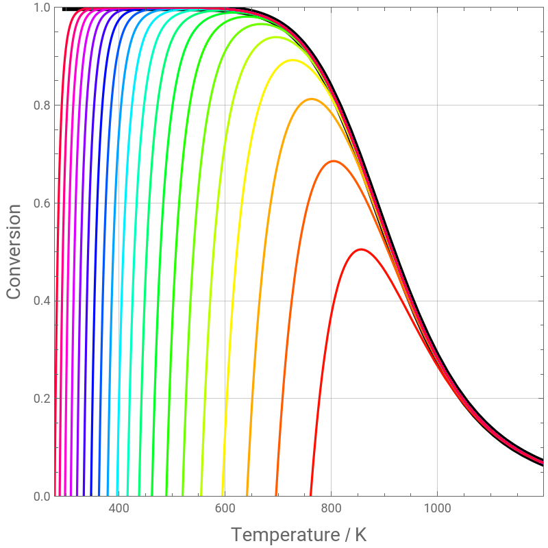
Conversion versus temperature for different values of the reaction rate.
j=0.01;
For[i=1,i<100,i+=1,j+=0.1;Sol[i]=Solve[Log[10,Rate]-j,X]]
tbl=Table[X/.Sol[i],{i,1,99}];
For[i=1,i<100,i+=5,Plt[i]=Plot[tbl[[i]],{T,200,1200},PlotRange->{0,1},PlotStyle->Hue[i/100]]]
We get the same result as figure 19.11 page 437 of O. Levenspiel, Chemical Reaction Engineering, 3rd Edition, Wiley, 1999.
pl=Show[plt,Flatten[Table[Plt[i],{i,1,99,5}]],PlotRange->{0,1},AspectRatio-> 1,FrameLabel->{Style["Temperature / K",14],Style["Conversion",14]},
ImageSize-> 400 {1,1},PlotRange->{{300,1200},{0,1}},Frame->True,GridLines->Automatic]
ImageSize-> 400 {1,1},PlotRange->{{300,1200},{0,1}},Frame->True,GridLines->Automatic]
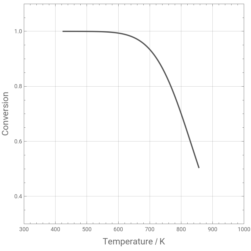
Finding the locus of optimum curve
Opt[i_]:=FindRoot[Flatten[D[X/.Sol[i],{T,1}]]0,{T,250,1700}]
tbl1=Table[T/.Opt[i],{i,1,99}];
tbl2=Flatten[Table[X/.Sol[i]/.Opt[i],{i,1,99}]];
tbl3=Transpose[{tbl1,tbl2}];
pl1=ListPlot[tbl3,PlotStyle->{Thick,Darker@Gray},PlotJoined->True,AspectRatio-> 1,FrameLabel->{Style["Temperature / K",14],Style["Conversion",14]},
ImageSize-> 400 {1,1},PlotRange->{{300,1000},{0.3,1.1}},Frame->True,GridLines->Automatic]
ImageSize-> 400 {1,1},PlotRange->{{300,1000},{0.3,1.1}},Frame->True,GridLines->Automatic]
Show[pl,pl1,PlotRange->{{400,1100},{0,1.05}}]
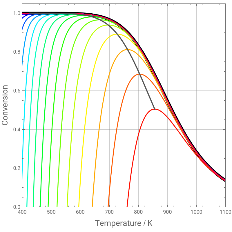
Interpolation of the optimum conversion versus temperature data
tbl4=Transpose[{tbl2,tbl1}];
rec=Interpolation[tbl4];
Computing optimum temperatures and rates for different conversions
Tbl={rec[0.46],rec[0.58],rec[0.66],rec[0.715],rec[0.785],rec[0.85]};
rate[X_,T_]:=(1-X)-X
299975.944190522`
T
7-
10067.356266538369`
T
18-
20134.712533076738`
T
rat=Thread[rate[{0.46,0.58,0.66,0.715,0.785,0.85},Tbl]];
flb=Transpose[{{0.46,0.58,0.66,0.715,0.785,0.85},1/rat}];
InvReactRate=InvReactRate=Interpolation[flb,InterpolationOrder 3];
Use of the method of maximization of rectangles to minimize the amount of catalyst needed in the two adiabatic packed bed system with very large recycle ratio (R=∞). We obtain figure E19.2b page 442 of O. Levenspiel, Chemical Reaction Engineering, 3rd Edition, Wiley, 1999.
PLT2=Plot[InvReactRate[x],{x,0.5,1},PlotRange{{0,1},{0,30}},AspectRatio-> 1,
FrameLabel->{Style["Conversion",14],Style["Inverse of Optimal Reaction Rate",14]},ImageSize-> 400 {1,1},Frame->True,GridLines->Automatic]
FrameLabel->{Style["Conversion",14],Style["Inverse of Optimal Reaction Rate",14]},ImageSize-> 400 {1,1},Frame->True,GridLines->Automatic]
sol2=FindRoot[InvReactRate'[ξ]-(20.59-InvReactRate[ξ])/(0-ξ),{ξ,5.5}]
y=(InvReactRate'[ξ]/.sol2) (x-ξ/.sol2)+InvReactRate[ξ]/.sol2
plt8=Plot[y,{x,0,1},PlotStyle->Darker@Cyan,AspectRatio-> 1,
ImageSize-> 400 {1,1},Frame->True,GridLines->Automatic]
ImageSize-> 400 {1,1},Frame->True,GridLines->Automatic]
plt7=Plot[{InvReactRate[ξ]/.sol2},{x,0,ξ}/.sol2,PlotStyle->{Thick,Black},PlotRange{{0,1},{0,25}},Filling->Axis,FillingStyleGreen]
plt6=Plot[{InvReactRate[0.85]},{x,ξ,0.85}/.sol2,PlotRange{{0,1},{0,25}},PlotStyle->{Thick,Black},Filling->Axis,FillingStyleOrange]
Show[plt6,plt7,plt8,PLT2,Graphics[{Darker@Cyan,Thick,Line[{{ξ,20.591}/.sol2,{0,InvReactRate[ξ]/.sol2}}]}],AspectRatio->1]
Conversion at exit of first reactor is ξ=0.670871 and Temperature is equal to 808K
ξ/.sol2
rec[ξ/.sol2]
Amount of catalyst needed in the two packed bed reactors are W1 and W2 and they are expressed in Kg.
W1=100 InvReactRate[ξ/.sol2] ξ/.sol2
W2=100 (InvReactRate[ξ/.sol2]-InvReactRate[0.85]) ((ξ/.sol2)-0.85)
Location and duty of heat exchangers. Three heat exchangers will be used to cool the system and their heat duties are equal to Q1, Q2 and Q3. Heat exchangers 1 and 2 will be placed in the recycle loop of the reactors.
Q1=100 ((808-300) 40-80000 0.6708)
Q2=100 ((750-808) 40-80000 (0.85-0.6708))
Q3=100 40. (300-750)
The recommended Design is given in the following sketch