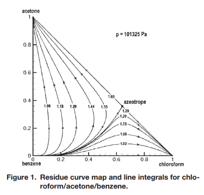
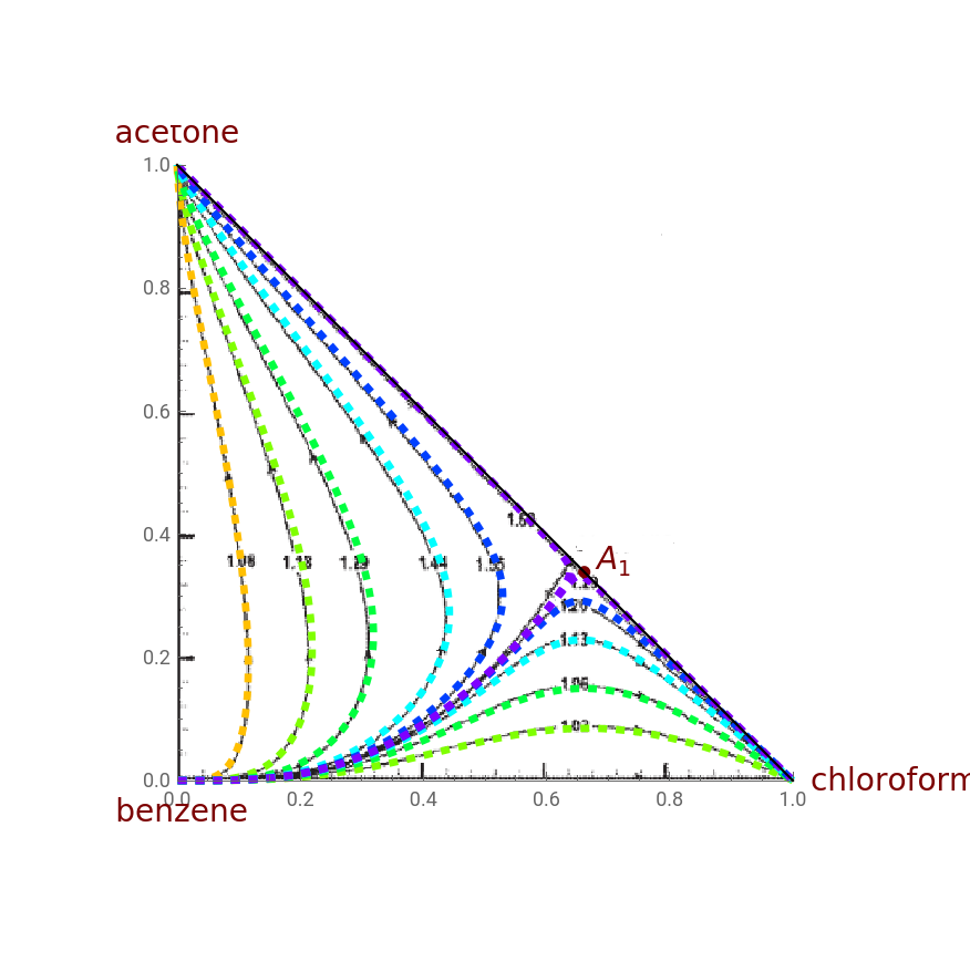
The objective of the present calculation is to reproduce Figure 1 given by Lucia and Taylor in 2006. In this later figure, Lucia provide a method to identify the unique distillation boundary that arises for the ternary system: chloroform (component 1) - acetone (component 2) - benzene (component 3). This distillation boundary corresponds to the residue curve that has the largest line integral. This boundary stems from the pure benzene apex of the triangular diagram and ends at the unique azeotrope of this system (noted as in our figure). is a binary azeotrope with coordinates as follows: {x1=0.6613, x2=0.3387}. The distillation boundary has a line integral equal to 1.69 and splits the domain into two regions (i.e., above and below this separation frontier). Following the work of Lucia (Ref. 1), we take the starting points for the calculation of any residue curve the point defined below : , where . Such coordinates depend on z. First, we determine the first set of z-values that will result in the residue curves (above the distillation boundary) with line integrals : {1.08,1.18,1.29,1.44,1.55,1.69}. Then, we determine the second set of z- values that will result in the residue curves (below the distillation boundary) with the line integrals : {1.02,1.06,1.13,1.20,1.29}. Using these specific values of z, we can compute the corresponding residue curves by integration using Euler’s method (integration step is 0.1) and NestList Command.The system obeys the there equations: =- for i=1..3 with ξ : the warped time.Finally, we compare our Residue Curve Map (RCM) to its counterpart given in Ref. 1. We get good agreement and the small discrepancies are most likely attributable to minor differences in the thermodynamic model.
A
1
A
1
(,)=×(cos(θ),sin(θ))
x
1
x
2
-3
10
θ=×zπ
1
2
-6
10
x
i
ξ
x
i
y
i
R=1.987;(*universalgasconstantinkcal/K*kmol*)P=760;(*totalpressureis760mmHg*)
Wilson model and Antoine equation
In[]:=
Aa1=6.95465;Ba1=1170.966;Ca1=226.232;Aa2=7.63132;Ba2=1566.69;Ca2=273.419;Aa3=6.87987;Ba3=1196.76;Ca3=219.161;Psat1=10^(Aa1-Ba1/(T+Ca1));Psat2=10^(Aa2-Ba2/(T+Ca2));Psat3=10^(Aa3-Ba3/(T+Ca3));l12=-506.85180;l21=116.11710;l13=-71.8108901977539;l31=-11.8231000900269;l23=682.406127929688;l32=-243.965103149414;V1=80.73;V2=74.47;V3=89.56;A12=V2/V1Exp[-l12/(R*(T+273.15))];A13=V3/V1Exp[-l13/(R*(T+273.15))];A32=V2/V3Exp[-l32/(R*(T+273.15))];A21=V1/V2Exp[-l21/(R*(T+273.15))];A31=V1/V3Exp[-l31/(R*(T+273.15))];A23=V3/V2Exp[-l23/(R*(T+273.15))];GAM1[x1_,x2_,x3_]:=Exp[-Log[x1+x2*A12+x3*A13]+1-(x1/(x1+x2*A12+x3*A13)+x2*A21/(x1*A21+x2+x3*A23)+x3*A31/(x1*A31+x2*A32+x3))];GAM2[x1_,x2_,x3_]:=Exp[-Log[x1*A21+x2+x3*A23]+1-(x1*A12/(x1+x2*A12+x3*A13)+x2/(x1*A21+x2+x3*A23)+x3*A32/(x1*A31+x2*A32+x3))];GAM3[x1_,x2_,x3_]:=Exp[-Log[x1*A31+x2*A32+x3]+1-(x1*A13/(x1+x2*A12+x3*A13)+x2*A23/(x1*A21+x2+x3*A23)+x3/(x1*A31+x2*A32+x3))];
Function RESIDU uses z as an argument and computes a residue curve
In[]:=
RESIDUE[z_?NumericQ]:=Module{f,p,theta,tbl1},theta=Piz210^-6;p={0,0}+10^-3{Cos[theta],Sin[theta]};f[{x1_,x2_,x3_}]:=x1+0.1-x1,x2+0.1-x2,x3+0.1-x3/.FindRoot[PGAM1[x1,x2,x3]Psat1x1+GAM2[x1,x2,x3]Psat2x2+GAM3[x1,x2,x3]Psat3x3,{T,60}];tbl1=Quiet[NestList[f,{p[[1]],p[[2]],1-p[[1]]-p[[2]]},450]];tbl1;
GAM1[x1,x2,x3]Psat1x1
P
GAM2[x1,x2,x3]Psat2x2
P
GAM3[x1,x2,x3]Psat3x3
P
Function length uses z as an argument and computes the line integral of the residue curve corresponding to z.
In[]:=
length[z_?NumericQ]:=Module{f,tbl1,distance,p,theta},theta=Piz210^-6;p={0,0}+10^-3{Cos[theta],Sin[theta]};f[{x1_,x2_,x3_}]:=x1+0.1-x1,x2+0.1-x2,x3+0.1-x3/.FindRoot[PGAM1[x1,x2,x3]Psat1x1+GAM2[x1,x2,x3]Psat2x2+GAM3[x1,x2,x3]Psat3x3,{T,60}];tbl1=Quiet[NestList[f,{p[[1]],p[[2]],1-p[[1]]-p[[2]]},450]];distance=Sum[Table[EuclideanDistance[{tbl1[[i,1]],tbl1[[i,2]]},{tbl1[[i+1,1]],tbl1[[i+1,2]]}],{i,1,449}][[j]],{j,1,449}];distance;
GAM1[x1,x2,x3]Psat1x1
P
GAM2[x1,x2,x3]Psat2x2
P
GAM3[x1,x2,x3]Psat3x3
P
Here we use the line integrals of Fig 1 by Lucia and Taylor in order to find the corresponding z-values
In[]:=
DATA1={1.08,1.18,1.29,1.44,1.55,1.69}
Out[]=
{1.08,1.18,1.29,1.44,1.55,1.69}
In[]:=
DATA2={1.02,1.06,1.13,1.20,1.29}
Out[]=
{1.02,1.06,1.13,1.2,1.29}
Let us compute the residue curves for the two region (i.e., above and below the distillation frontier)
We take advantage of the Parallel Computing capability of Mathematica in order to decrease computational time.
We take advantage of the Parallel Computing capability of Mathematica in order to decrease computational time.
Plotting the RCM
Finally, we compare our data with those of Fig. 1 (Ref. 1)
Reference
Reference
◼
[1] Angelo Lucia and Ross Taylor . "The geometry of separation boundaries: I. Basic theory and numerical support," 52 (2), pp . 582–594, 2006.
CITE THIS NOTEBOOK
CITE THIS NOTEBOOK
Residue Curve Map for the Ternary System: Chloroform - Acetone - Benzene
by Housam Binous and Ahmed Bellagi
Wolfram Community, STAFF PICKS, January 31, 2024
https://community.wolfram.com/groups/-/m/t/3113178
by Housam Binous and Ahmed Bellagi
Wolfram Community, STAFF PICKS, January 31, 2024
https://community.wolfram.com/groups/-/m/t/3113178