The billiard problem examines the motion of a particle freely traveling within a closed, bounded region and undergoing elastic reflections at its boundary. Key questions focus on whether the particle eventually visits all regions and travels in all possible directions. Using Birkhoff coordinates, the system’s dynamics can be analyzed via a two-dimensional Poincaré return map. The orbits observed in this phase space range from periodic closed paths to invariant curves and chaotic trajectories. This computational study leverages the Wolfram Language to simulate billiard dynamics and investigate the diverse orbit structures that emerge. This computational essay is a quick review and implementation of a seminal paper by Sir Michael Berry, “Regularity and chaos mechanics, illustrated in classical by three deformations of a circular ‘billiard’”.
Berry, M V, 1981, Eur.J.Phys 2, 91-102
Berry, M V, 1981, Eur.J.Phys 2, 91-102
Functions
Functions
Theory
Theory
A “billiard problem” consist of a particle moving freely in a region defined by a plane bounded by a closed curve and being reflected elastically (=) at the impacts with . This condition preserves the particle’s energy, meaning that its position and direction of motion are the only essential parameters determining its state.
α
reflection
α
incidence
Main questions on billiard problems are:
◼
After many bounces, the particle visited the neighbourhood of every point within ?
◼
Has the particle travelled in almost every direction?
To answer this questions, we can analyze the various types of orbits generated by the billiard.
The billiard flow has a natural Poincaré section defined by Birkhoff coordinates with the arclength position of the n-th bounce measured along the billiard boundary, and =pCos[] the momentum component parallel to the boundary, where is the angle between the outgoing trajectory and the normal to the boundary. Without loss of generality, we set . The Poincaré section condition and energy conservation () reduces the Poincaré section map P to two dimensions. Finally, the dynamics are given by the return map ,) , ) from the -th collision to the -th collision.
{,}
s
n
p
n
s
n
p
𝑛
α
α
𝑛
m=v=p=1
p=1
P:(
s
n
p
n
(
s
n+1
p
n+1
n
(n+1)
In the Birkhoff phase space, the various types of orbits form a discrete and area-preserving mapping and can be catalogue as:
◼
Closed (Zero-dimensional): The system repeatedly returns to a finite set of points.
◼
Invariant curve (One-dimensional): The whole curve maps onto itself under P.
◼
Chaotic (two-dimensional): The orbit fills an area in a chaotic manner.
In this computational essay, we demonstrate how the Wolfram Language can be used to simulate this type of system and explore the emergent orbits that arise from its dynamics.
Functionalities example
Functionalities example
Define the curve parametrization:
In[]:=
ClearAll[,][θ_,δ_]:=Sin[θ]+δ/2Sin[θ]+δ/6Sin[3θ];[θ_,δ_]:=-Cos[θ]+δ/2Cos[θ]-δ/6Cos[3θ];
All the functionalities depend on and definitions, for example the position r:
In[]:=
δ0=;r[0,δ0]
9
10
Out[]=
0,-
7
10
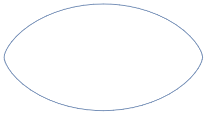
Which we can use to define a ParametricRegion
In[]:=
exampleOval=ParametricRegion[r[θ,δ0],{{θ,0,2π}}]//Region
Out[]=
Now, use bounceEvolution to start the billiard dynamics:
In[]:=
initialPositon=r[π/3,δ0];initialDirection={π/2,-π};example=bounceEvolution[initialPositon,initialDirection,δ0,"Bounces"->3];
Let’s check the result
In[]:=
example
Out[]=
Result,-,,-π,{{0.993357,0.399761},{0.9893,-0.145894}},{{-0.528048,0.624125},{0.748533,0.663098}},{{-1.29009,-0.0509434},{-0.996894,0.0787611}},PhaseSpace{{0.516467,-0.886826},{2.10612,-0.906582},{3.19371,-0.391164}}
29
3
40
1
8
π
2
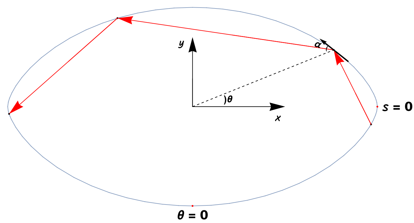
KeyValues for “Result” return a list of pair of vectors {, } and “PhaseSpace” returns a lit of pair of values .
position
n
direction
n
{,Cos()}
n
α
n
The following graphic shows the parameters used to analyze the system:
In[]:=
ShowexampleOval,Graphics[{Point/@#,Red,Arrow/@Partition[#,2,1]}]&@example["Result"][[All,1]],
Out[]=
Circle
Circle
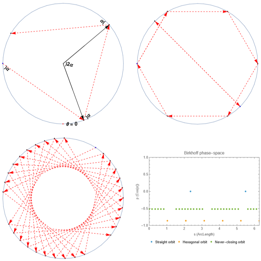
In a circle, the radius of the curve does not depend on the angle θ, then neither the reflecting angle α. Circular billiard motion is therefore restricted by the simple
conservation law
conservation law
p=constant
In this case, all curves would be invariant curves parallel to the direction. This behaviour occurs, if the dynamics is integrable meaning that there exists a constant of motion satisfying:
s
n
F(,)=F(,)
s
1
p
1
s
0
p
0
in which case the invariant curves are the contours of . If the dynamics are integrable, the case for chaotic orbits are excluded.
F(s,p)
Let’s define the parametrization for the circle curve:
In[]:=
ClearAll[,][θ_,δ_]:=Cosθ-;[θ_,δ_]:=Sinθ-;
π
2
π
2
In[]:=
regCircle=ParametricRegion[r[θ,0],{{θ,0,2π}}];
Using the following initial conditions, let’s observe the evolution of the billiard:
In[]:=
circlepaths=bounceEvolution[#[[1]],#[[2]],0,"Bounces"->#[[3]]]&/@{{r[3π/2,0],{1,-0.7},3},{r[π/4,0],AngleVector[3π/4],2},{r[-π/2,0],AngleVector[π/3],7},{r[π/2+1,0],AngleVector[π/7],30}};
In this case we expect to observe invariant curves and closed orbits (finite sets):
coordinates=("Result"/.circlepaths)[[All,All,1]];circlegraphics=Graphics&/@coordinates;circleplot=ListPlot"PhaseSpace"/.circlepaths[[2;;]],;GraphicsGridPartitionShow{Region@regCircle,#[[1]]},,Show[{Region@regCircle,#[[2]],#[[3]]}],Show[{Region@regCircle,#[[4]]}],circleplot,UpTo[2],ImageSize->&@circlegraphics
2.9
10
Out[]=
Stadium
Stadium
We propose an interesting parametrization called oval-billiard curve:
This parametrization will be helpful to easily obtain the shape deformation from circles to stadium.
Evolve the system using the following parameters:
Let’s observe the results:
It is also worth to mention that those “holes” are connected with the family of two-bounce closed orbits formed by perpendicular impacts on the straight sections of the stadium:
Ellipse
Ellipse
The billiard motion in an ellipse is always integrable, which generate a lot of contrast with the stadium curve that generated ergodic motion. The constant of motion is given by:
where ϵ is the ellipse eccentricity.
Define the parametrization for the ellipse curve :
Using above formula, we can visualize how the contours of the phase space will look like using the defined constant of motion:
For this curve we observe two possible orbits, the rotator and librator. This is because each orbit will repeatedly touch a conic confocal with :
◼
An ellipse
◼
An hyperbola
Let’s check the results, we expect to obtain a rotator touching the ellipse and a librator touching the hyperbola:
Understanding this, we can test various initial conditions to generate sufficient closed orbits and invariant curves, allowing us to verify that our results align with the contours of the constant of motion:
Oval
Oval
The previously analyzed curves are not considered “generic” or “typical” boundaries because those represent specific cases designed to illustrate different orbits in the phase space of the billiard problem. In contrast, the oval boundary exhibits generic behavior, meaning that all the different types of orbits we previously described coexist within it.
Define the following parametrization for the oval curve :
Four-bounce anticlockwise orbit
Four-bounce anticlockwise orbit
When talking about four-bounce anticlockwise circulating orbits, circles an ellipses present a continuous family of trajectories. As an integrable system, this means that perturbation lead to nearby orbits. In contrast, ovals present the property that all closed orbits are isolated, then we can only find two distinct four-bounce orbits: an stable and unstable orbit.
Unstable and stable orbits
Unstable and stable orbits
Define the parameters and region for our example:
Execute the experiment for this initial conditions:
Let’s analyze the results:
Magnification
Magnification
The richest behavior is found around the unstable orbit. In the magnification of this section of the phase space, we find a chaotic area surrounding the unstable closed orbits, which is a generic feature of them. Between the stable and unstable orbits we can find elongated “islands”. Islands emergence also shows that structures repeat recursively down to infinitely fine scales.
In the following image we can observe important features of the system structure:
◼
Invariant curves around stable fixed points
◼
Chaos around unstable fixed points
Transition from Rotation to Chaos
Transition from Rotation to Chaos
Chaotic regions emerge from trajectories that repeatedly focus on two specific points within the oval boundary:
Complete plot
Complete plot
The resulting plot reveals many of the characteristics discussed in the previous sections. We observe chaotic behavior resembling a diffuse, dust-like version of the unstable orbits, along with islands forming between regions of stable and unstable orbits.
Complete plot
Complete plot
The resulting plot highlights many of the characteristics discussed in the previous sections. We observe chaotic behavior, often referred to as a “chaos ocean”, which leaves distinct empty regions. These gaps will gradually be filled as the number of bounces approaches infinity, in accordance with the ergodic theorem.
References
References
◼
Berry, M.V. (1981) ‘Regularity and chaos in classical mechanics, illustrated by three deformations of a circular “billiard”’
European Journal of Physics, 2(2), pp. 91–102.
https://iopscience.iop.org/article/10.1088/0143-0807/2/2/006
European Journal of Physics, 2(2), pp. 91–102.
https://iopscience.iop.org/article/10.1088/0143-0807/2/2/006
◼
P. Cvitanović, R. Artuso, R. Mainieri, G. Tanner and G. Vattay (2020) Chaos: Classical and Quantum,
Niels Bohr Institute, Copenhagen
https://chaosbook.org/
Niels Bohr Institute, Copenhagen
https://chaosbook.org/
◼
LEONEL, E.D. (2022) Scaling laws in dynamical systems.
SPRINGER VERLAG, SINGAPOR
https://link.springer.com/book/10.1007/978-981-16-3544-1
SPRINGER VERLAG, SINGAPOR
https://link.springer.com/book/10.1007/978-981-16-3544-1
CITE THIS NOTEBOOK
CITE THIS NOTEBOOK
Billiard dynamics: from regularity to chaos
by Sebastian Rodriguez
Wolfram Community, STAFF PICKS, February 11, 2025
https://community.wolfram.com/groups/-/m/t/3391864
by Sebastian Rodriguez
Wolfram Community, STAFF PICKS, February 11, 2025
https://community.wolfram.com/groups/-/m/t/3391864