Introduction
Introduction
This notebook is an attempt to model airflow past a moving vehicle. It implements a 2D CFD model using Mathematica’s FEM capabilities.
A wind tunnel is modeled in the frame of reference in which the car is at rest, with the following boundary conditions:
◼
The inlet has a uniform horizontal inflow of 60 mph representing the vehicle speed
◼
The output has a defined pressure of 0 Pa.
◼
The top is an open boundary with no restrictions.
◼
The bottom represents the road and has a fixed horizontal airspeed equal to the inlet speed, since it is non-slip in the frame of reference in which the car is at rest and the road is in motion.
◼
The car boundaries are non-slip, with zero boundary airspeed in both directions.
Issues
Issues
In the first implementations of this notebook NDSolve would not converge. This did not surprise me in that the system being modeled has a high Reynolds Number, at least bordering on turbulent conditions.
I therefor implemented a parametric continuation sweep to try to acquire convergence by a sequence of solutions. In this implementation, a scaling parameter is defined which allows a sequence of solutions to begin with a system having a low Reynolds number, and proceed one step at a time toward the desired system. In this process, the solution for each system becomes the initial seed for NDSolve as it tries to solve the system for a new value of the scaling parameter. Since the Reynolds number of the system is proportional to the fluid density, the scaling parameter is implemented as a unitless constant which multiplies the air density. The sweep begins with a small value for the scaling parameter. The goal is to step-by-step achieve convergence with the scaling parameter equal to 1.
One thing that surprises me in the results:
The largest parameter for which I obtained a converged solution is 0.00057. This represents a Reynolds number which is an extremely low fraction of the intended system. In fact, in another implementation of this notebook, where I defined the system using a Reynolds number parameter (how is that implemented?), the largest number for which I obtained a converged solution was 9. This is deep in the laminar flow regime. (And the results look laminar.) I would think that Reynolds numbers in the hundreds could be solved. Perhaps this could be done with a more refined use of FEM options, and finer meshes do seem to improve convergence. One reason I post this is the hope that I might obtain advice on this from those with greater knowledge.
Questions
Questions
1
.Solution convergence improves with finer mesh. Are there ways to improve meshing without impractical solution times on computing equipment I can afford? Examples from other tools include the ability to separately define meshes adjacent to boundaries, or to make use of automatic mesh refinement in areas where an initial solution identifies strong gradients.
2
.Are there other solvers or solver parameters that might improve the ability of NDSolve to converge? For example, other algorithms or better control of adaptive stepping.
3
.Are there other ways to present the problem to Mathematica which offer better convergence?
Preliminaries
Preliminaries
In[]:=
$Version
Out[]=
14.2.1 for Microsoft Windows (64-bit) (March 17, 2025)
In[]:=
Needs["NDSolve`FEM`"]$HistoryLength=0;
In[]:=
SetDirectory[NotebookDirectory[]];
Constants
Constants
Units are MKS
In[]:=
μAir=1.789*^-5;(*viscosity*)ρAir=1.225;(*density*)
In[]:=
recLength=50;recHeight=15;carx=15;carLength=5;carHeight=2;cary=0.25;rad=.5;speed=QuantityMagnitude@UnitConvert60,//N;
Region
Region
In[]:=
car=ResourceFunction["RoundedPolygon"][{{carx,cary},{carx+carLength,cary},{carx+carLength,carHeight},{carx,carHeight}},rad];
In[]:=
rec=Rectangle[{0,0},{recLength,recHeight}];
In[]:=
Ω=RegionDifference[rec,car];
In[]:=
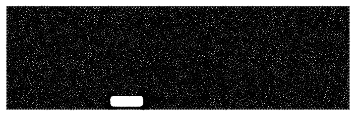
mesh=ToElementMesh[Ω,MaxCellMeasure->.1];mesh["Wireframe"]
Out[]=
Set up and solve the PDE
Set up and solve the PDE
In[]:=
vars={{u[x,y],v[x,y],p[x,y]},{x,y}};
Boundaries
Boundaries
In[]:=
(*outletboundaryat0pressure*)outletPressure=0;
In[]:=
outlet=DirichletCondition[p[x,y]outletPressure,x==recLength];
In[]:=
(*inlethasuniforminflow*)inlet=DirichletCondition[{u[x,y]==speed,v[x,y]==0},x0];
In[]:=
(*roadmoveswithspeedofflowandboundaryisnoslip*)road=DirichletCondition[{u[x,y]==speed,v[x,y]==0},y==0];
In[]:=
(*carisnoslip*)carBoundary=DirichletCondition[{u[x,y]==0,v[x,y]==0},carx<=x<=carx+carLength&&cary<=y<=carHeight];
In[]:=
(*topisopenboundary*)
In[]:=
(*combinedboundaryconditions*)bcs={outlet,inlet,road,carBoundary};
Continuation sweep function
Continuation sweep function
This is the continuation sweep function. It accepts the scaling factor k and solves the PDE using nextSeed as the initial seed. If it succeeds, it saves a next seed for the next iteration. If it fails it aborts.
In[]:=
solve[k_]:=Module[{},(*printtemporaryasprogressindicator*)NotebookDelete[temp];temp=PrintTemporary["k factor = ",k];(*thecontinuationparameter*)kn=k;(*notethatthedensityofairismultipliedbytheparameter*)pars=<|"DynamicViscosity"->μAir,"MassDensity"->knρAir|>;(*solvethepdewithaninitailseed*)pde=FluidFlowPDEComponent[vars,pars]=={0,0,0};sol={uVel,vVel,pressure}=NDSolveValue[{pde,bcs},vars[[1]],{x,y}∈mesh,Method{"FiniteElement","InterpolationOrder"{u->2,v2,p1}},InitialSeeding->nextSeed];(*ifthesolutionisnotalistthenithasfailed,soprintandabort*)If[!Head[sol]===List,Print["k factor = ",k," failed"];Abort[]];(*solutionisvalid--formatitasthenextseed*)nextSeed=MapThread[Equal,{{u[x,y],v[x,y],p[x,y]},{uVel,vVel,pressure}}];(*andsavethevalidsolutionforuseafterafailure*)lastSol=sol;]
Perform continuation sweep
Perform continuation sweep
Consecutive sweeps will be made with increasing values of the scaling function k until the sweep function aborts.
In[]:=
(*intializenextSeedforthefirstiteration*)nextSeed={u[x,y]==speed,v[x,y]==0,p[x,y]==outletPressure};
In[]:=
(*callsolvewithincreasingvaluesfork*)Quiet[Do[solve[k],{k,.00001,1,.00001}]]
k factor = 0.00058 failed
Out[]=
$Aborted
In[]:=
(*savethelastsuccessfulsolutiontoafilesowecanworkonpostprocessingwithoutrerunningthesimulations*)DumpSave["lastSol.mx",lastSol];
PostProcessing
PostProcessing
In[]:=
(*loadthesolutionincaseweneedit*)<<"lastSol.mx"
In[]:=
{uVel,vVel,pressure}=lastSol;
Plots
Plots
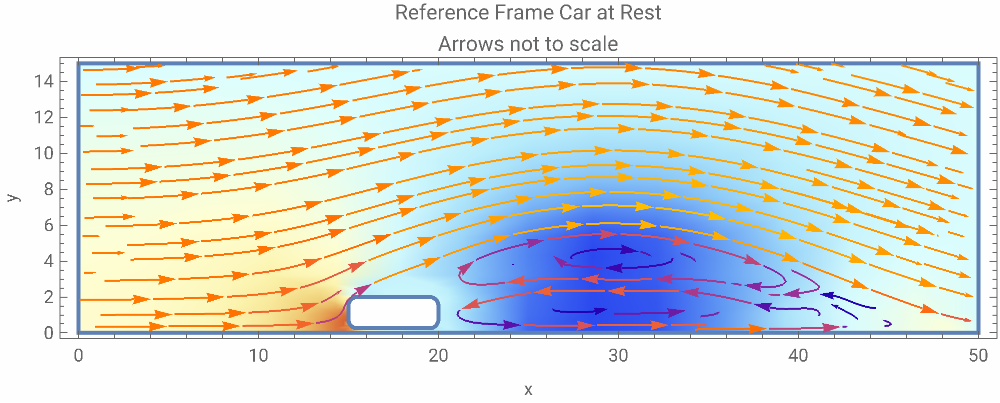
As the model was implemented, the car was at rest but the air and road were moving
In[]:=
Show[{DensityPlot[pressure,{x,y}∈mesh,Sequence[ColorFunction->"LightTemperatureMap",PlotLegends->Placed[BarLegend[Automatic,LegendLabel->"p(x,y)"],Bottom],PlotRange->All]],StreamPlot[{uVel,vVel},{x,y}∈mesh,Sequence[StreamPoints->Fine,RegionFillingStyle->None]]},Sequence[FrameLabel->{"x","y"},ImageSize->500],AspectRatio->Automatic,PlotLabel->"Reference Frame Car at Rest\nArrows not to scale"]
Out[]=

In[]:=
VectorPlot[{uVel,vVel},{x,y}∈mesh,AspectRatio->Automatic,VectorScalingAutomatic,VectorSizes->{.5,2},VectorPoints->{20,10},ImageSize->500,PlotLegends->Placed[BarLegend[Automatic,LegendLabel->"Airflow Speed"],Below],PlotLabel->"Reference Frame Car at Rest"]
Out[]=
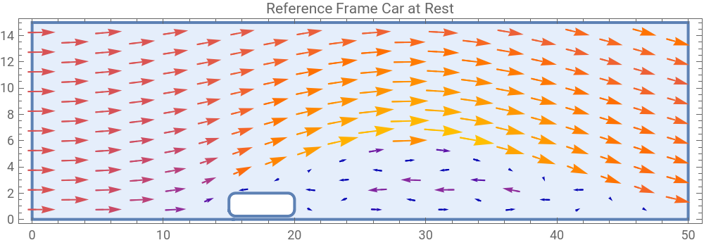

Subtracting the inlet air speed from the result gives the result in the frame of reference of the road, where the car is moving.
Forces
Forces
If we integrate the inward unit normal vector multiplied by the local air pressure over the boundary of the car we get the force applied to the car by airflow. Or we would, if we actually solved the problem in 3D with the correct density for air.
Cite This Notebook
Cite This Notebook
Modeling Airflow Past a Car
by David Keith
Wolfram Community, July 10, 2025
by David Keith
Wolfram Community, July 10, 2025