Ternary Liquid Liquid Equilibrium using a Combination of Common Tangent Plane and Arc-Length Continuation
Authors: Housam Binous
Ternary Liquid Liquid Equilibrium using a Combination of Common Tangent Plane and Arc-Length Continuation
Authors: Housam Binous
Authors: Housam Binous
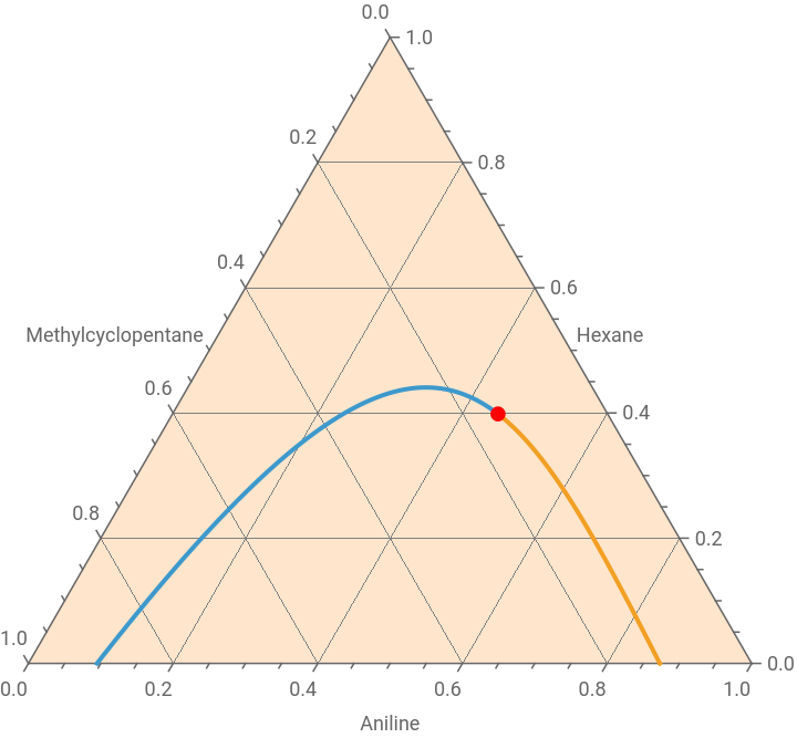
The liquid–liquid equilibrium (LLE) behavior of the ternary aniline–hexane–methylcyclopentane system at 45 °C was investigated using the Non-Random Two-Liquid (NRTL) activity-coefficient model. The equilibrium compositions were determined through an arc-length continuation technique applied to the common tangent conditions of the Gibbs free energy of mixing surface.
The calculation was initiated from a composition pair located near the plait point, obtained by solving the common tangent equations with a small distance parameter (d=0.001). This solution served as the starting point for the continuation procedure. An arc-length constraint was then introduced, allowing the system of nonlinear algebraic equations to be transformed into a differential-algebraic system and solved continuously using NDSolve. The continuation parameter enabled stable tracing of the entire binodal curve while avoiding convergence difficulties typically encountered near critical solution points.
The resulting ternary phase diagram exhibits Type-I liquid–liquid equilibrium behavior, characterized by a single closed miscibility gap and the presence of a plait point. The red point shown in the figure corresponds to the calculated plait point, where the compositions of the two coexisting liquid phases become identical. The smooth continuation of both branches of the binodal curve demonstrates the robustness and numerical stability of the arc-length method.
The results confirm that the combination of the NRTL thermodynamic model and arc-length continuation provides an efficient and reliable framework for calculating ternary liquid–liquid equilibria and accurately locating critical solution points in partially miscible systems.
Method based on common tangent plane
In[]:=
ClearAll["Global`*"];R=1.9872041;(*universalgasconstant*)T=273.15+45;(*temperature*)(*NRTLPARAMETERS*)param={a13->0.3,a12->0.20,a32->0.30,B12->857.3718000,B21->2650.684300,B13->1410.932300,B31->2291.817900,B23->190.1605000,B32->-153.9573000,A12->-1.969300000,A13->-2.802700000,A23->0.0,A21->-7.132100000,A31->-5.248600000,A32->0.0};t13=A13+B13/T;t23=A23+B23/T;t12=A12+B12/T;t32=A32+B32/T;t31=A31+B31/T;t21=A21+B21/T;α={{0.,a12,a13},{a12,0.,a32},{a13,a32,0.}}/.param;τ={{0.,t12,t13},{t21,0.,t23},{t31,t32,0.}}/.param;
In[]:=
α//MatrixForm
Out[]//MatrixForm=
0. | 0.2 | 0.3 |
0.2 | 0. | 0.3 |
0.3 | 0.3 | 0. |
In[]:=
τ//MatrixForm
Out[]//MatrixForm=
0. | 0.725567 | 1.6321 |
1.19946 | 0. | 0.597707 |
1.95498 | -0.483914 | 0. |
In[]:=
G[i_,j_]:=Exp[-α[[i,j]]τ[[i,j]]];(*COMPOSITIONVECTOR*)xvec[x1_,x2_]:={x1,x2,1-x1-x2};(*NRTLACTIVITYCOEFFICIENTS*)lnGamma[i_,x1_,x2_]:=Module[{x,term1,term2},x=xvec[x1,x2];term1=Sum[x[[j]]τ[[j,i]]G[j,i],{j,1,3}]/Sum[x[[k]]G[k,i],{k,1,3}];term2=Sum[x[[j]]G[i,j]/Sum[x[[k]]G[k,j],{k,1,3}](τ[[i,j]]-Sum[x[[m]]τ[[m,j]]G[m,j],{m,1,3}]/Sum[x[[m]]G[m,j],{m,1,3}]),{j,1,3}];term1+term2];gamma[i_,x1_,x2_]:=Exp[lnGamma[i,x1,x2]];(*DIMENSIONLESSGIBBSENERGYOFMIXING:g/RT*)gmix[x1_,x2_]:=Module[{x},x=xvec[x1,x2];Sum[x[[i]]Log[x[[i]]],{i,1,3}]+Sum[x[[i]]lnGamma[i,x1,x2],{i,1,3}]];(*DERIVATIVES*)dgdx1[x1_,x2_]:=Evaluate[D[gmix[u,v],u]/.{u->x1,v->x2}];dgdx2[x1_,x2_]:=Evaluate[D[gmix[u,v],v]/.{u->x1,v->x2}];(*UNKNOWNS*)vars={x1a,x2a,x1b,x2b,m1,m2};(*COMMONTANGENTEQUATIONS*)eq1=dgdx1[x1a,x2a]==m1;eq2=dgdx1[x1b,x2b]==m1;eq3=dgdx2[x1a,x2a]==m2;eq4=dgdx2[x1b,x2b]==m2;eq5=gmix[x1b,x2b]-gmix[x1a,x2a]==m1(x1b-x1a)+m2(x2b-x2a);(*EXTRACONSTRAINT-Preventtrivialsolutionxα=xβ*)eq6=(x1b-x1a)^2+(x2b-x2a)^2==d;
In[]:=
(*firstvalueford---verysmalld=0.001yieldapproximatelytheplaitpoint*)d0t=0.001;
In[]:=
(*solution*)solct=FindRoot[{eq1,eq2,eq3,eq4,eq5,eq6/.d->d0t},{{x1a,0.1},{x2a,0.20},{x1b,0.70},{x2b,0.2},{m1,0.45},{m2,0.5}},MaxIterations->1000]
Out[]=
{x1a0.43817,x2a0.405496,x1b0.465024,x2b0.388797,m10.924659,m20.533594}
In[]:=
init={x1a[0]==(x1a/.solct),x2a[0]==(x2a/.solct),x1b[0]==(x1b/.solct),x2b[0]==(x2b/.solct),m1[0]==(m1/.solct),m2[0]==(m2/.solct),d[0]==d0t}
Out[]=
{x1a[0]0.43817,x2a[0]0.405496,x1b[0]0.465024,x2b[0]0.388797,m1[0]0.924659,m2[0]0.533594,d[0]0.001}
In[]:=
initdev={x1a'[0]==0.01,x2a'[0]==0.01,x1b'[0]==0.01,x2b'[0]==0.01,m1'[0]==0.01,m2'[0]==0.01,d'[0]==0.01}
Out[]=
{[0]0.01,[0]0.01,[0]0.01,[0]0.01,[0]0.01,[0]0.01,[0]0.01}
′
x1a
′
x2a
′
x1b
′
x2b
′
m1
′
m2
′
d
In[]:=
SYS={eq1,eq2,eq3,eq4,eq5,eq6}/.x1a->x1a[s]/.x1b->x1b[s]/.x2a->x2a[s]/.x2b->x2b[s]/.m1->m1[s]/.m2->m2[s]/.d->d[s];
In[]:=
Length@init
Out[]=
7
In[]:=
Length@initdev
Out[]=
7
In[]:=
Length[SYS]
Out[]=
6
In[]:=
auxeq=x1a'[s]^2+x1b'[s]^2+x2a'[s]^2+x2b'[s]^2+m1'[s]^2+m2'[s]^2+d'[s]^2==1
Out[]=
2
′
d
2
′
m1
2
′
m2
2
′
x1a
2
′
x1b
2
′
x2a
2
′
x2b
In[]:=
SYSFinal=Join[SYS,{auxeq},init,initdev];
In[]:=
Length@SYSFinal
Out[]=
21
In[]:=
SOL=NDSolve[SYSFinal,{x1a,x2a,x1b,x2b,m1,m2,d},{s,-100,100}]

Out[]=
x1aInterpolatingFunction,x2aInterpolatingFunction,x1bInterpolatingFunction,x2bInterpolatingFunction,m1InterpolatingFunction,m2InterpolatingFunction,dInterpolatingFunction


In[]:=
DATA1=Table[{x1a[s],x2a[s],1-x1a[s]-x2a[s]}/.SOL,{s,-17.7,0.020,0.01}];DATA2=Table[{x1b[s],x2b[s],1-x1b[s]-x2b[s]}/.SOL,{s,-17.7,0.020,0.01}];
In[]:=
Pt={{2,1},{0,Sqrt[3.]}}/2;
Type I liquid-liquid equilibrium (LLE) diagram - Plait point indicated in red
In[]:=
p0=Show[TernaryListPlot[{Flatten[DATA1,1],Flatten[DATA2,1]},Joined->True,PlotStyle->Thick,GridLines->Automatic,FrameLabel->{"Aniline","Hexane","Methylcyclopentane"},PlotRange->All,Method->{"Backdrop"->LightOrange}],Graphics[{Red,PointSize[0.02],Point[Pt.{x1a[s],x2a[s]}/.SOL/.s->0.020]}]]
Out[]=