ORIGINAL ARTICLE: Takatoshi Yamada, (2022), Practical numerical solutions of Wassermann–Wolf equations, Optik. 257: 168725. https://doi.org/10.1016/j.ijleo.2022.168725
Article abstract: In this paper, we present a complete method for determining the two surfaces of an aspheric singlet by numerical integration based on the classical Wassermann–Wolf equations (hereinafter WW). Although aplanatic optics is mainly treated in WW, we also show some other examples that can be determined by the WW. This indicates that surface shape determination by optimization software such as Zemax or CodeV is not necessary for some aspherical singlet designs, including the aplanatic case. A link to an executable Mathematica code for this purpose is also provided.
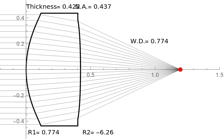
Aplanatic aspherical singlet design demonstration
Aplanatic aspherical singlet design demonstration
The surface shapes of both sides are fixed by numerically solving the Wassermann-Wolf equation. The focal length always normalized to 1.0. You can specify some parameters, numerical aperture, lens thickness, CSF (Coddington Shape Factor that represents lens bending), wavelength and glass medium (extracted from SCHOTT catalog). Some sets of the parameters can not reach solutions with specified N.A. For these cases, this notebook shows maximum N.A. under the specified paraxial conditions.


Contents
Contents
This notebook summarizes the derivation of expressions in the original paper,
“Practical numerical solutions of Wassermann–Wolf equations”:
https://doi.org/10.1016/j.ijleo.2022.168725
“Practical numerical solutions of Wassermann–Wolf equations”:
https://doi.org/10.1016/j.ijleo.2022.168725
This notebook contains derivations of :
1. Wassermann-Wolf equations from Snell’s law 2. explicit equations for infinite conjugate singlet 3. explicit equations for infinite conjugate singlet with a cover glass 4. explicit equations for finite conjugate singlet without cover glasses 5. explicit equations for finite conjugate singlet with cover glass in the image space 6. explicit equations for finite conjugate singlet with cover glass in the object space 7. explicit equations for finite conjugate singlet with cover glass in both spaces 8. explicit equations for afocal singlet 9. explicit equations for one-dimensional Gaussian-to-tophat converter 10. explicit equations for pseudo-Bessel beam generator
Please also refer the classical Wassermann–Wolf equations (hereinafter WW) paper :
Wassermann G.D., Wolf E.
“On the theory of aplanatic aspheric systems” Proc. Phys. Soc. B, 62 (1) (1949), p. 2
“On the theory of aplanatic aspheric systems” Proc. Phys. Soc. B, 62 (1) (1949), p. 2
Notations
Notations
in WW, symbols concerning the second surface are specified by adding dash "'" but in Mathematica "'" symbol is used for derivative of Lagrange' s notation.
Therefore, subscript is used for assigning surfaces, e.g.,
Therefore, subscript is used for assigning surfaces, e.g.,
In[]:=
{[t],[t],[t]};
ω
1
ω
s
ω
2
mean
ω,,ω'
*
ω
in WW.
And all Mathematica symbols defined by the author are started by small case characters because we can easily distinguish them from system symbols.
In Mathematica, dependent variables are better to be expressed explicitly with independent variable,e.g.,
In[]:=
ω[t];
not
In[]:=
ω;
Deriving Wassermann-Wolf equation
Deriving Wassermann-Wolf equation
Preliminarily, Snell’s law in parametric surface expression
Preliminarily, Snell’s law in parametric surface expression
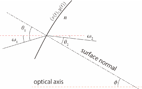
Here is well known Snell' s law expression.
Please put your insertion cursor inside the text box bellow and then input shift-return key to evaluate the expression.
After the evaluation, your Mathematica kernel has learned the expression for later use.
After the evaluation, your Mathematica kernel has learned the expression for later use.
In[]:=
snellsLaw=(*Sin[]*Sin[]);
n
1
θ
1
n
2
θ
2
Please check the prompt header changed to “In[1]:=” from “In[*]:=” after evaluation.
Hereafter please evaluate text boxes with prompt “In[*]:=” in turn.
And please be careful that the order of evaluation may affect the results.
Hereafter please evaluate text boxes with prompt “In[*]:=” in turn.
And please be careful that the order of evaluation may affect the results.
transforming it from the figure above,
In[]:=
replaceAngles={-ϕ,-ϕ};replaceSurfaceNormalAngle=(ϕArcTan[-x'[t]/y'[t]]);
θ
1
ω
1
θ
2
ω
2
leads the same mathematical meaning as an expression in Eq.(2.5) of WW. assuming y[t] is monotonous and concerning part of surface axis above
In[]:=
Simplify[TrigExpand[snellsLaw/.replaceAngles]/.replaceSurfaceNormalAngle,{Element[{x'[t]},Reals],y'[t]>0}]
Out[]=
n
1
ω
1
′
x
ω
1
′
y
n
2
ω
2
′
x
ω
2
′
y
The equation above is same meaning of Snell’s law expressed in Eq.(2.5) of WW, also same as Eq.(1) in the original paper.
Start from Snell's law for each surfaces, Eq.(2.5) in WW.
Start from Snell's law for each surfaces, Eq.(2.5) in WW.
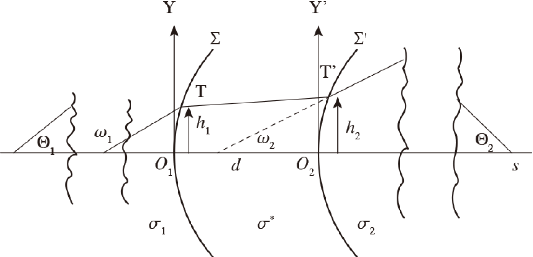
From here, dependent variables of 't' are expressed explicitly, i.e., ‘f[t]’ not ‘f’.
In[]:=
snell
1
n
1
ω
1
x
1
ω
1
y
1
ω
s
x
1
ω
s
y
1
snell
2
n
2
ω
2
x
2
ω
2
y
2
ω
s
x
2
ω
s
y
2
y dependency formulae, Eq.(2.8) and (2.9) in WW.
In[]:=
yDependencies[baseExpression]={[t][t]+[t]Tan[[t]],[t][t]+[t]Tan[[t]]};
y
1
h
1
x
1
ω
1
y
2
h
2
x
2
ω
2
and their derivatives
In[]:=
yDependencies[differentials]=Map[D[#,t]&,yDependencies[baseExpression]];
R definitions, Eq.(2.6) and Eq.(2.7) in WW.
In[]:=
omegaAstariscs={Sin[[t]]/R,Cos[[t]]/R};vectorRDefinition={->[t]-[t]+d,[t]-[t],RSqrt[^2+^2]};
ω
s
R
y
ω
s
R
x
R
x
x
2
x
1
R
y
y
2
y
1
R
x
R
y
Rewrite expressions for derivative of x1 and x2 to get the equivalents to Eq.(2.10) and Eq.(2.11) in WW
In[]:=
wweq1011[original]=Thread[{'[t],'[t]}==Flatten[{'[t],'[t]}/.Simplify[Solve[{,}/.yDependencies[differentials]/.omegaAstariscs,{'[t],'[t]}]]]]
x
1
x
2
x
1
x
2
snell
1
snell
2
x
1
x
2
Out[]=
[t]-,[t]-
′
x
1
(RSin[[t]]-n)([t]+[t][t])
ω
1
n
1
R
y
′
h
1
2
Sec[[t]]
ω
1
x
1
′
ω
1
RSec[[t]]-n(+Tan[[t]])
ω
1
n
1
R
x
R
y
ω
1
′
x
2
(RSin[[t]]-n)([t]+[t][t])
ω
2
n
2
R
y
′
h
2
2
Sec[[t]]
ω
2
x
2
′
ω
2
RSec[[t]]-n(+Tan[[t]])
ω
2
n
2
R
x
R
y
ω
2
For confirmation of the equivalency, the first factor of Eq.(2.10) in WW.
For confirmation of the equivalency, the first factor of Eq.(2.10) in WW.
before that, a preparatory helper function : fractionalRationalize[_,_]
In[]:=
Clear[fractionalRationalize];fractionalRationalize[fraction_,factor_]:=Apply[Divide,Map[Expand[#*factor]&,NumeratorDenominator[fraction]]]
here is a denominator factor of Eq.(2.10) and Eq.(2.11) in WW
In[]:=
originalFirstFactor=1/((n*-R*Cos[ω[t]])/(n*-R*Sin[ω[t]])+Tan[ω[t]])
R
x
R
y
Out[]=
1
-RCos[ω[t]]+n
R
x
-RSin[ω[t]]+n
R
y
In[]:=
Simplify[Map[Together,originalFirstFactor]]
and the second factor of Eq.(2.10)
lead the expression above.
Further calculation beyond Schwarzschild example in WW.
Further calculation beyond Schwarzschild example in WW.
Initial conditions
Initial conditions
and explicit expression of θ (t)
Hereafter, all singlets is in air.
Deriving equations for infinite conjugate singlet
Deriving equations for infinite conjugate singlet
The first example is an infinite conjugate lens.
It's an easy geometric exercise.
It's an easy geometric exercise.
Eq.(2.10) and Eq.(2.11) in WW (equivalent expressions Eq(1) and Eq.(2) in the original) are derived only from Snell’s law, therefore the equations does not include conditions of stigmatism or aplanatism apparently.
Sine conditions or stigmatism need to formularize separately from WW equations as conditions for ray congruence.
The desired expressions for the infinite conjugate singlet can be obtained by substituting the conditions of the ray congruence into the equations.
transform to an explicit expression about variable t, eliminating dependencies with θ,ω etc...
The expressions are rather large and It is difficult to solve them analytically because it is nonlinear.
Trying to solve with numerical values by evaluating the equation above.
Trying to solve with numerical values by evaluating the equation above.
The standard function “NDSolve” can be used to solve this simultaneous nonlinear differential equations
And “ParametricPlot” function can be used to show the solved lens shape.
Infinite conjugate singlet with cover glass
Infinite conjugate singlet with cover glass
Same as above except existence of a cover glass in the object space, right-side of a lens.
Same as above except existence of a cover glass in the object space, right-side of a lens.
The ray congruence rules bellow include the refraction at the both surfaces of the cover glass.
transforming to an explicit expressions
evaluating the expressions numerically
and plot.
Finite Conjugate
Finite Conjugate
Next example is a finite conjugate case.
Ray congruence conditions :
Then the numerical solution can be obtained :
Finite conjugate with cover glass in image space
Finite conjugate with cover glass in image space
Next example is a finite conjugate case with a cover glass.
evaluation of an expression bellow may be slow.
Finite conjugate with cover glass in object space
Finite conjugate with cover glass in object space
Next example is a finite conjugate case with a cover glass but it is in object space.
evaluation of an expression bellow may also be slow.
Finite conjugate with cover glass in both image and object space
Finite conjugate with cover glass in both image and object space
Next example is a finite conjugate case with a cover glass in both space.
This configuration is commonly seen on optical disc pickups, i.e., an objective lens with a beam splitter and disc.
This configuration is commonly seen on optical disc pickups, i.e., an objective lens with a beam splitter and disc.
It may take very log time to evaluate the expression bellow because it will be very large.
But it can be numerically solved.
Afocal singlet
Afocal singlet
The next example is an afocal optics by aspherical singlet lens. It may only be used for beam expander, etc...?
The next example is an afocal optics by aspherical singlet lens. It may only be used for beam expander, etc...?
All previous examples were completely aplastic singlets. However, the WW equations do not contain aplanatism in the equation itself, as mentioned earlier. Therefore, the equations and their methods above can be applied other optical design cases.
Combination of the equations and the ray congruence rules can also be solved numerically.
Tophat converter
Tophat converter
An example of afocal system case.
An example of afocal system case.
Laser beam with gaussian profile is converted to tophat (flat - top) profile by the converter . This example is two-dimensional, in z-y plane. This case is not rotational symmetric but the equations and the methods can accept the case.
From two-dimensional geometrical intensity conservation,
leads a differential equation,
Bessel beam generator
Bessel beam generator
The other non-aplanatic example.
The other non-aplanatic example.
Pseudo - Bessel beam can be produced by an axicon lens. This pseudo-Bessel beam generator example is better to get longer focal depth and working distance. The solution is rotational symmetric, not two-dimensional.
From three- dimensional geometrical intensity conservation, for small area ds,
where Ii(h) and Io(h2(h)) are intensities at height h respectively.
It leads a differential equation,
It leads a differential equation,
From total intensity conservation,the constant Υ0 can be determined,
And fix the constant of integration from the inside most ray,
Take positive solution,
Check the solution to lead marginal relation,
Angle in the image space ω1 be set to a constant κ.
Conclusion
Conclusion
WW equations and “NDSolve” function of Mathematica should have applications other than aplanatic lenses as shown in the afocal optics or the Bessel beam generator.
CITE THIS NOTEBOOK
CITE THIS NOTEBOOK
Practical numerical solution of Wassermann - Wolf equations
by Takatoshi Yamada@AYASE Co.,Ltd.
Wolfram Community, STAFF PICKS, March 21, 2022
https://community.wolfram.com/groups/-/m/t/2494155
by Takatoshi Yamada@AYASE Co.,Ltd.
Wolfram Community, STAFF PICKS, March 21, 2022
https://community.wolfram.com/groups/-/m/t/2494155