Wolfram Mathematica Integration techniques Roger Wells 2023 July Mathematicians welcome . . . all others . . . BOW YOUR HEADS! Still working on how to make the Plus C appear +-Log[x]Integrate:Unknown option GeneratedParameters in Integrate-+3x+,x,GeneratedParametersC.Symbolic Computer Algebra Quadratic roots, discriminant, directrix plots . . . very powerful. Integrate the function (x) cos (x) dx and plot the new function calling it . . . Trex Using the assignment operator Trex := Learn the tools and artwork. Aspect Ratio Golden Ratio RANGE in mathematica does mean the typical “y” value (the ordinate) and Domain (from algebra . . . “abscissa”) is a set or list of arguments . . . the x axis. Be prudent on this to make great scientific documents, with pleasing and elegant mathematical arguments . . . for the human eye. Wolfram mathematica Shift + drag midpoint (not corner) handle to stretch and shrink plot Using the Aspect Ratio of 2 means the Range to Domain ratio is two to one This is what it means to say a movie has been formated to your screen. In fact a television movie is usualy “formated” the other way around . . . width to hieghth. An aspect Ratio of 1 means square 1 x 1 This of course is the perfect “ picture” for exact math functions . . . “one to one”. Typos intended. And of course the Golden Ratio which is how mathematica displays a plot by default is The abscissa to ordinate ratio Continue to explore a function by re-naming it . . . Z Z : = Plot [ Z ] { x , 0 , 2 Pi } ] Wolfram mathematica Determine the integral from minus 2 π and 2 π for the function Sine ( π x ) dx.Sin[πx]x
∫x^4+3x-
1
x
Integrate[x^4+3x-1/x,x]

3
2
x
2
5
x
5
Integrate+3x-,x,GeneratedParametersC
4
x
1
x

1
x
4
x
Integrate[a+bx+c,x]
2
x
cx++
b
2
x
2
a
3
x
3
Integrate[Sin[x]^2*Cos[x],x]
3
Sin[x]
3
2
sin
Trex:=
3
Sin[x]
3
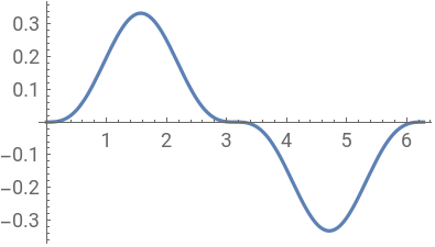
Plot[Trex,{x,0,2∏}]
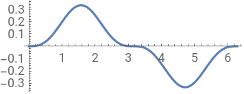
Plot,{x,-8,8}
3
Sin[x]
3

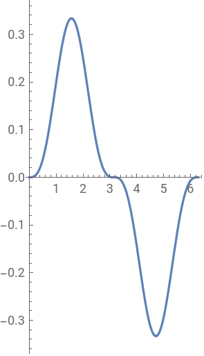
Plot,{x,0,2Pi},AspectRatio2
3
Sin[x]
3
1+√5
2
1-Cos[]
2
π
π
π
∫
0
Plot,{x,-2Pi,2*Pi},AspectRatio1
1-Cos[]
2
π
π
1-Cos[]
2
π
π
Plot,{x,-2Pi,2*Pi},AspectRatio12
1-Cos[]
2
π
π
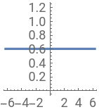
Plot,{x,-2Pi,2*Pi},AspectRatio2
1-Cos[]
2
π
π
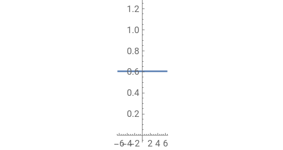
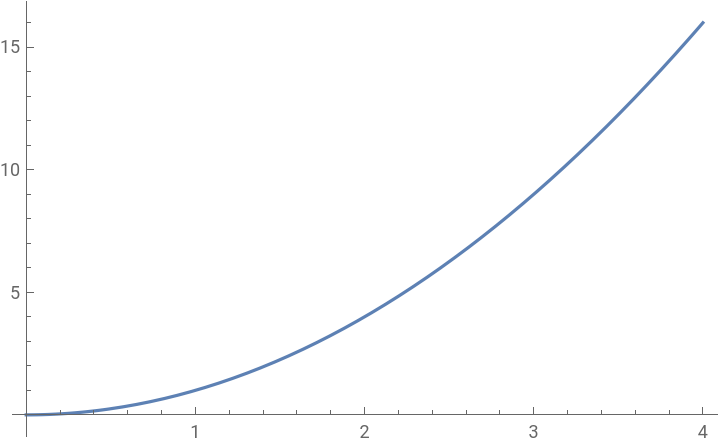
f[x_]:=
2
x
g[x_]:=2x
Plot[f[x],{x,0,4}]