Particle in Infinite Potential Well: Analytical vs Numerical
Particle in Infinite Potential Well: Analytical vs Numerical
A. Samsonyan
Wolfram Labaratory, Russian-Armenian University, Yerevan, Armenia
In our laboratory we are engaged in numerical modeling of processes in nanostructures, using Wolfram Language. In particular, we study optical and light phenomena to quantum dots, such as: interband absorption, photoluminescence, intraband absorption, nonlinear absorption, harmonic generations in quantum dots and much more. In this paper, we will show how to compare numerical and analytical results.
Introduction
Introduction
The study of the energy spectrum of quantum dots represents a key task in the field of nanosystems physics and quantum technologies. These nanoscale structures, functioning as artificial atoms, exhibit a discrete energy level spectrum due to the quantum confinement of charge carriers. Two primary approaches are used for the theoretical investigation of such systems: analytical methods, based on exact solutions of model problems, and numerical methods, which provide accurate results under complex geometries and realistic conditions.
Comparing analytical and numerical results allows researchers to evaluate the accuracy of the applied models, identify their limitations, and gain a deeper understanding of the underlying physical processes in quantum dots. While analytical approaches offer valuable physical insight and help to establish general principles, numerical methods deliver precision and flexibility in modeling complex systems.
A special role in numerical modeling is played by Wolfram Mathematica — a versatile platform that combines symbolic and numerical analytical tools. It enables solving the Schrödinger equation with various potential configurations using finite-difference methods and variational techniques. Moreover, Mathematica offers powerful visualization tools that significantly aid in interpreting results. Its ability to create adaptive numerical algorithms makes it an indispensable tool for research in nanophysics and quantum mechanics.
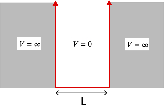
In this paper we consider the behavior of a particle in an infinitely deep potential well and compare analytically accurate calculations with numerical simulations (Figure below).
Comparing analytical and numerical results allows researchers to evaluate the accuracy of the applied models, identify their limitations, and gain a deeper understanding of the underlying physical processes in quantum dots. While analytical approaches offer valuable physical insight and help to establish general principles, numerical methods deliver precision and flexibility in modeling complex systems.
A special role in numerical modeling is played by Wolfram Mathematica — a versatile platform that combines symbolic and numerical analytical tools. It enables solving the Schrödinger equation with various potential configurations using finite-difference methods and variational techniques. Moreover, Mathematica offers powerful visualization tools that significantly aid in interpreting results. Its ability to create adaptive numerical algorithms makes it an indispensable tool for research in nanophysics and quantum mechanics.
In this paper we consider the behavior of a particle in an infinitely deep potential well and compare analytically accurate calculations with numerical simulations (Figure below).
Comparison
Comparison
The analytical solution for the particle in a infinite quantum well problem is fairly well known and has the following form:
In[]:=
ClearAll[eigensystemAnalytical];eigensystemAnalytical[L_, n_] :=
Next we carry out standard numerical modeling:
In[]:=
ClearAll[eigensystemNumerical];eigensystemNumerical[L_, n_, method_] :=
Of course, a very important point is the choice of a numerical modeling method. In this paper we considered the following methods based on eigensystem or eigenvalues:
Out[]=
or other numverical methods:
Out[]=
It is clear that the final goal is to identify the wave function and energy for both the analytical and numerical cases and compare them.
We have the simplest task, when we have dependencies only on the well length and the quantum state of the particle (in the numerical case, of course, the numerical calculation methods we considered earlier are added).
We have the simplest task, when we have dependencies only on the well length and the quantum state of the particle (in the numerical case, of course, the numerical calculation methods we considered earlier are added).
Out[]=
Energy
Wave Function
Density Plot
Analytic vs Numerical
