A general parabola on the complex plane with polar coordinates can be constructed by multiplying the polar radius by and and adding a complex focus. θ is the parametric parameter in radians, α is a rotation angle in radians, and F = h + k is the location of the focus. There is a discontinuity at θ = 2 π n, where n is an integer. A solution is developed in polar coordinates to draw a parabola through any four points on a plane.
θ
α
In[]:=
Clear["Global`*"];radius=p/(1-Cos[θ]);F=h+Ik;rotation=Exp[Iα];
The general complex formula is constructed, where Z is a complex point on a parabola:
In[]:=
Z=rotationradiusExp[Iθ]+F
Out[]=
h+k+p
α+θ
1-Cos[θ]
Real valued vector form can be recovered with ComplexExpand.
In[]:=
ComplexExpand[Z]
Out[]=
h++k+
pCos[α+θ]
1-Cos[θ]
pSin[α+θ]
1-Cos[θ]
The same formula can be derived with real valued vectors.
In[]:=
RotationMatrix[α].{radiusCos[θ],radiusSin[θ]}+{h,k}//TrigReduce
Out[]=
,
-h+hCos[θ]-pCos[α+θ]
-1+Cos[θ]
-k+kCos[θ]-pSin[α+θ]
-1+Cos[θ]
A complex polar formula for a straight line is below, where α is an angle Normal to the line and p is the distance from the line to the origin. The same parameters can be used in parametric Cartesian coordinates with the second formula,
In[]:=
line=+;
2p
(α+2θ)
2α
2θ
Note that the formula disappears at p = 0, consequently a line cannot be plotted through the origin, but it can plot the directrix of a parabola with the focus at the origin.
With trigonometric polar coordinates:
With trigonometric polar coordinates:
In[]:=
ComplexExpand[line]//Simplify//Expand;{Re[#][[1]],Im[#][[1]]}&@@%
Out[]=
{pCos[θ]Sec[α-θ],pCos[θ]Sec[α-θ]}
Here is a visualization of the formula for a parabola with Manipulate, using what has been developed above. To match the line formula with the directrix, -line is used as p is negative with respect to the F.
In[]:=
ManipulateShowParametricPlotReImxy[[1]]+Ixy[[2]]+p,ReIm-++xy[[1]]+Ixy[[2]],{θ,0,2Pi},PlotRange->{{-25,25},{-25,25}},Epilog->{Black,PointSize[0.02],Point@{xy[[1]],xy[[2]]}},Plot[xy〚2〛+(x-xy〚1〛)Tan[α+Θ],{x,-40,40},PlotStyle->{Black,Thickness[0.0035]},AspectRatio->Automatic],GraphicsRed,PointSize[0.02],PointReImxy1+xy2+p,PointReImxy1+xy2+p,Black,LineReImxy1+xy2+p,ReImxy1+xy2-p+Cos[α]Imp-RepSin[α],Line-Im[xy〚2〛]+Rep+xy1,Imp+xy1+Re[xy〚2〛],-Im[xy〚2〛]+Rexy1-p+Cos[α]Imp-RepSin[α],Imxy1-p+Cos[α]Imp-RepSin[α]+Re[xy〚2〛],{{α,0},0,2Pi,Appearance->"Labeled"},{{p,5},1/20,20},{{xy,{0,0}},{-5,-5},{5,5}},{{Θ,0+10^-6},0+10^-6,2Pi+10^-6},SaveDefinitions->True
α+θ
1-Cos[θ]
2p
(α+2θ)
2α
2θ
α+Θ
1-Cos[Θ]
α+(π+Θ)
1+Cos[Θ]
α+Θ
1-Cos[Θ]
α
(α+Θ)
-1+Cos[Θ]
(α+Θ)
-1+Cos[Θ]
α+(π+Θ)
1+Cos[Θ]
α+(π+Θ)
1+Cos[Θ]
α
(π+α+Θ)
-1-Cos[Θ]
(π+α+Θ)
-1-Cos[Θ]
α
(π+α+Θ)
-1-Cos[Θ]
(π+α+Θ)
-1-Cos[Θ]
Out[]=


Manipulate diagram observations:
Θ is the angle on the complex plane, where the focus is at the origin. When α is greater than 0, the black line is at an angle, Θ + α. Θ on the graphic corresponds to the black line through the focus at angle, θ + α in the formula, intersecting the parabola at red points. The formula cannot plot at θ = 0, which would be the vertex angle, α. At every non-zero value for θ, the line at the angle θ + α through the focus intersects the parabola at two points, corresponding to the values for θ and θ + Pi, which makes it a straight line. The distance between the focus and a point on the parabola is equal to the distance to the directrix line (orange).
Θ is the angle on the complex plane, where the focus is at the origin. When α is greater than 0, the black line is at an angle, Θ + α. Θ on the graphic corresponds to the black line through the focus at angle, θ + α in the formula, intersecting the parabola at red points. The formula cannot plot at θ = 0, which would be the vertex angle, α. At every non-zero value for θ, the line at the angle θ + α through the focus intersects the parabola at two points, corresponding to the values for θ and θ + Pi, which makes it a straight line. The distance between the focus and a point on the parabola is equal to the distance to the directrix line (orange).
Parabola diagram
Parabola diagram
The code is described in more detail in the next section. The code has a different naming to prevent conflicts between calculated points and formula points.
In[]:=
parm=<|α->Pi/3,p->1,h->1,k->1|>;theta=Pi/3;line=+;directrix=-line+F;k-Imp+-h+x+RepTan[α];zLine=Imh-p+Re[k]+x+Im[k]-Re[h]+RepTan[α];vertexLine=k+(-h+x)Tan[α];directrixLine=k-(-h+x+pCos[α])Cot[α]-pSin[α];ZD=h+k-p+p(-Cos[α]+Sin[α])Cos[θ]Im+ReSin[θ];PP=h-pCos[α]+(k-pSin[α])/.parm;
2p
(α+2θ)
2α
2θ
(α+θ)
-1+Cos[θ]
(α+θ)
-1+Cos[θ]
(α+θ)
-1+Cos[θ]
(α+θ)
-1+Cos[θ]
α
1
-1+Cos[θ]
1
-1+Cos[θ]
In[]:=
prange={{-2,5},{-2,5}};PG=Graphics[{Blue,PointSize[0.015],Point[ReIm[PP]]/.parm}];ZG=Graphics[{Darker@Green,PointSize[0.015],Point[ReIm[Z]]/.parm/.θ->theta}];circleG=Graphics[{ColorData[97][3],Circle[ReIm[Z],Abs[Z-F]]/.parm/.θ->theta}];line0G=Graphics[{ColorData[97][3],Line[{ReIm[Z],ReIm[F]}]/.parm/.θ->theta}];zparabolaG=ParametricPlot[Evaluate[{ReIm[directrix],ReIm[Z]}/.parm],{θ,-Pi,Pi},PlotRange->prange,Epilog->{ColorData[97][4],PointSize[0.015],Point@ReIm[F]/.parm}];cPlotG=Plot[{vertexLine/.parm,directrixLine/.parm,zLine/.parm/.θ->theta},{x,-20,20},AspectRatio->Automatic];ZDG=Graphics[{Black,PointSize[0.015],Point@ReIm[ZD]/.parm/.θ->theta}];line1G=Graphics[{Black,Line[{ReIm[F],ReIm[ZD]}]/.parm/.θ->theta}];FF=F;ZZ=Z;txt=Block[{F,Z},Graphics[{Text["F",ReIm[FF]/.parm,{-3,0}],Text["Z",ReIm[ZZ]/.parm/.θ->theta,{-3,0}],Text["P",ReIm[PP]/.parm,{-3,0}],Text["Q",ReIm[ZD]/.parm/.θ->theta,{3,0}]}]];
In[]:=
Show[zparabolaG,circleG,line0G,cPlotG,ZG,ZDG,line1G,PG,txt]
Out[]=
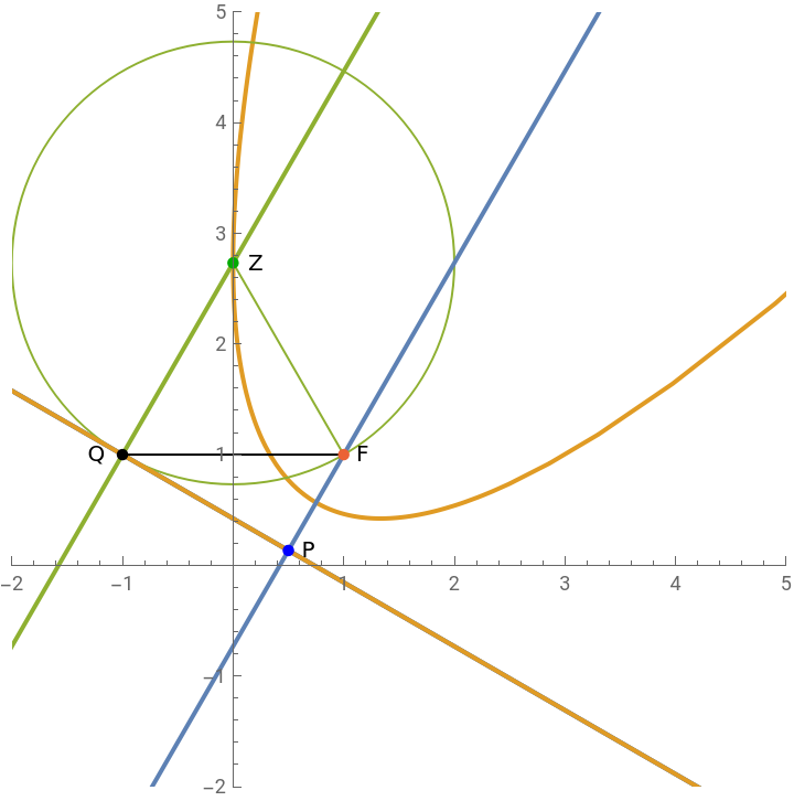
Parabola as a locus of points on complex plane.
Parabola as a locus of points on complex plane.
In the course of drawing the graphic above all the equations were solved to create complex points which demonstrate that a parabola is the locus of points equidistant from a F and a line, the directrix. With complex numbers the absolute value of the difference of two points is equal to the distance between the points and the Arg of a point gives its angle with respect to the plane. Translation is simply accomplished by adding or subtracting another complex number. For plotting lines it is easier to work with Cartesian coordinates.
The point P is at the intersection of the vertexLine and the directrixLine.
zLine, the perpendicular to the directrix through Z was calculated while making the diagram. Q is at the intersection of zLine and the directrixLine.
The graph of a parabola is given by the formula for Z; the point F was defined, and the point, Q, calculated.
The distance ZF equals the distance ZQ everywhere on the curve Z .
Polar four point solution
Polar four point solution
I started this project with the hope that a simple four point solution for a parabola with polar coordinates would fall off the tree, by using the complex plane. It turned out to be more difficult and the formulas I found don’t work well with Solve. A hybrid solution using Cartesian coordinates ultimately gives a solution.
Where
Then p1 is the formula Z
Isolate the imaginary parts
Eliminate the imaginary values so all numbers are in reals.
Eliminate the denominator; this equation could be used with zf z - h - k
Change to Cartesian coordinate system
Use four known points with the complex formula to test the algorithm.
End note
End note
The algorithm PolarParabola4Pt gives polar solutions for a parabola given four points, with parameters that Archimedes could understand. I could not find a polar parabola solution for four input points on internet searches, but I do not have access to academic library search. If anyone knows of another polar solution, I would appreciate a reference.
CITE THIS NOTEBOOK
CITE THIS NOTEBOOK
Parabola on the complex plane
by R. H. Rimmer
Wolfram Community, STAFF PICKS, November 22, 2023
https://community.wolfram.com/groups/-/m/t/3069438
by R. H. Rimmer
Wolfram Community, STAFF PICKS, November 22, 2023
https://community.wolfram.com/groups/-/m/t/3069438